2  Preliminaries: Communicating Systems and Games

The core background of this thesis is the trinity of characterizations for behavioral equivalences: relational, modal, and game-theoretic.

This chapter takes a tour into the field of formalisms used to model programs and communicating systems, which are accompanied by many notions for behavioral equivalence and refinement to relate or distinguish their models.

The tour is agnostic, building on the basic formalism of labeled transition systems and standard equivalences such as trace equivalence and bisimilarity. Simultaneously, the approach is opinionated, focusing on Robin Milner’s tradition of concurrency theory with a strong pull towards game characterizations.

Figure 2.1 shows the scaffold of this section along the trinity, instantiated to the classic notion of bisimilarity:

• Section 2.2 introduces (among other notions) bisimilarity through its relational characterization in terms of symmetric simulation relations.
• Section 2.3 treats the dual connection of bisimilarity and the distinguishing powers of a modal logic, known as the Hennessy–Milner theorem.
• Section 2.4 shows that both, the relations to validate bisimilarity and the modal formulas to falsify it, appear as certificates of strategies in a reachability game where an attacker tries to tell states apart and a defender tries to prevent this.

Figure 2.1: Core-correlations for bisimilarity between relational definition, modal distinguishability, and equivalence game.

Readers familiar with the contents of Figure 2.1 might mostly skim through this chapter of preliminaries (although they are quite exciting!). The two core insights this chapter aims to seed for the upcoming chapters are:

Idea 2.1: It’s all a game!

Equivalence games are a most versatile way to handle behavioral equivalences and obtain decision procedures. The Hennessy–Milner theorem appears as a shadow of the determinacy of the bisimulation reachability game.

Idea 2.2: Modal first!

Modal characterizations allow a uniform handling of the hierarchy of equivalences. Productions in grammars of potential distinguishing formulas translate to game rules for equivalence games.

Both points might seem non-standard to those more accustomed to relational or denotational definitions of behavioral equivalences. To provide them with a bridge, we will start with relational and denotational definitions—but once we have crossed this bridge, we will not go back.

2.1 Behavior of Programs

Every computer scientist has some model in their head of what it is that their algorithms and programs are doing. Usually these models are wrong,¹ especially, once concurrency enters the picture. The area of formal methods tries to make models sufficiently precise that one at least can say what went wrong.

¹ But some are useful, as the saying goes.

2.1.1 Labeled Transition Systems

Labeled transition systems are the standard formalism to discretely express the state space of programs, algorithms, and more. One can think of them as nondeterministic finite automata where the finiteness constraint has been lifted.

Definition 2.1 (Transition Systems) A labeled transition system (LTS) $\mathcal{S}=(\mathcal{P},\mathit{Act},\xrightarrow{\smash{\raisebox{-2pt}{$\scriptstyle{}$}}})$ consists of

• $\mathcal{P}$, a set of states,
• $\mathit{Act}$, a set of actions, and
• ${\xrightarrow{\smash{\raisebox{-2pt}{$\scriptstyle{}$}}}} ⊆ \mathcal{P}× \mathit{Act}× \mathcal{P}$, a transition relation.²

locale Labeled_Transition_Systems.lts

We write $\operatorname{Der}(p, α)$ for the set of derivative states $\{p' \mid p \xrightarrow{\smash{\raisebox{-2pt}{$\scriptstyle{α}$}}} p'\}$, and $\operatorname{Ini}(p)$ for the set of enabled actions $\{α \mid \exists p' \ldotp p \xrightarrow{\smash{\raisebox{-2pt}{$\scriptstyle{α}$}}} p'\}$.

There is a canonical example used to discuss equivalences within transition systems, which we want to draw from. We will take the formulation that Henzinger used at CAV’23 as seen in Figure 2.2.

Figure 2.2: Tom Henzinger employing Example 2.1 during CAV’23.

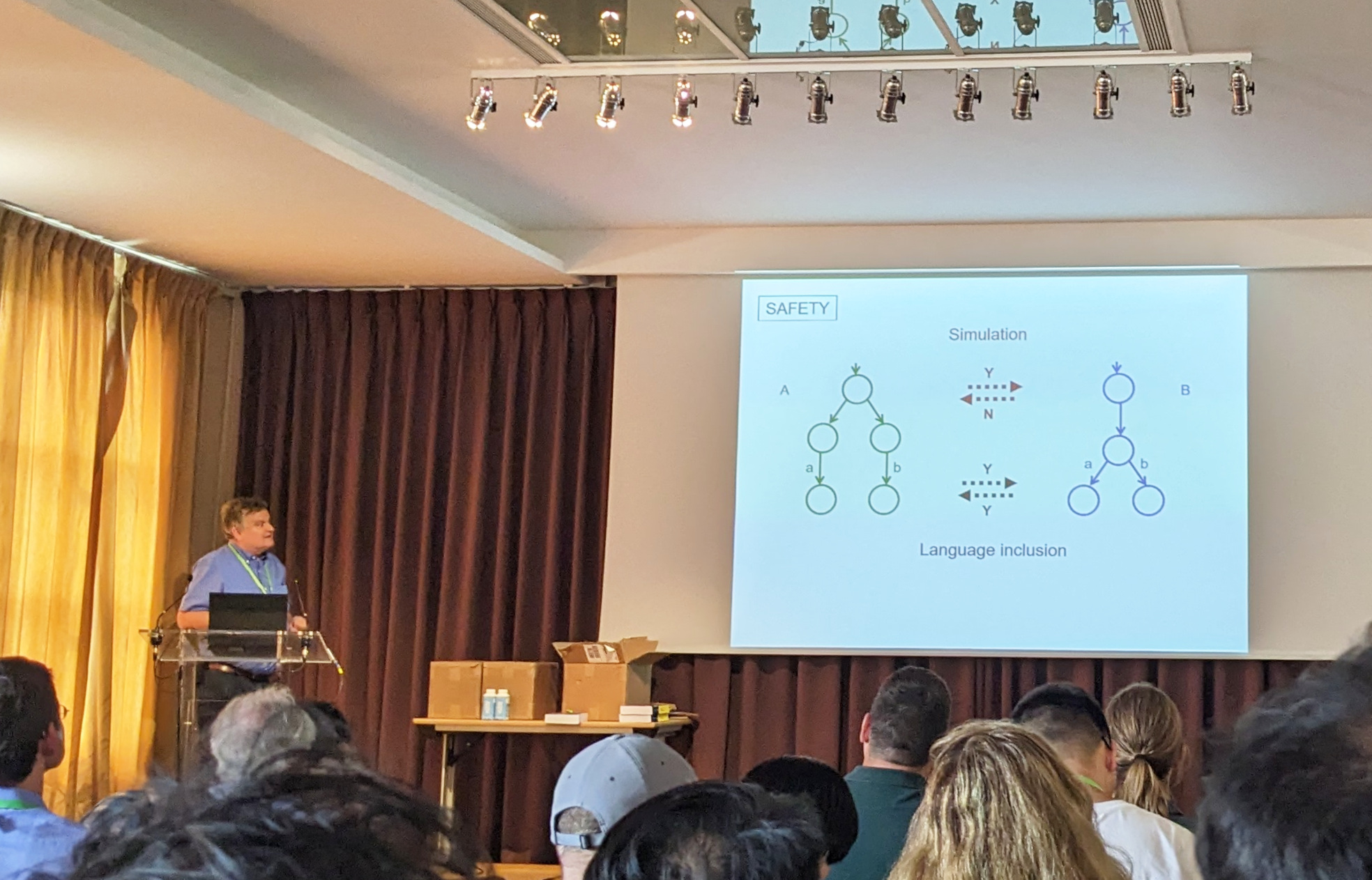
Example 2.1 (A Classic Example) Consider the transition system $\mathcal{S}_\mathsf{PQ} = (\{\mathsf{P}, \mathsf{p_a}, \mathsf{p_b}, \mathsf{p_1}, \mathsf{p_2}, \mathsf{Q}, \mathsf{q_{ab}}, \mathsf{q_1}, \mathsf{q_2}\}, \{\mathsf{a}, \mathsf{b}, τ\}, \xrightarrow{\smash{\raisebox{-2pt}{$\scriptstyle{\cdot}$}}}_\mathsf{PQ})$ given by the following graph:

Figure 2.3: Example system $\mathcal{S}_\mathsf{PQ}$.

The program described by the transitions from $\mathsf{P}$ chooses non-deterministically during a $τ$-step between two options and then offers only either $\mathsf{a}$ or $\mathsf{b}$. The program $\mathsf{Q}$ on the other hand performs a $τ$-step and then offers the choice between options $\mathsf{a}$ and $\mathsf{b}$ to the environment.

There are two things one might wonder about Example 2.1:

1. Should one care about non-determinism in programs? Subsection 2.1.2 shows how non-determinism arises naturally in concurrent programs.
2. Should one consider $\mathsf{P}$ and $\mathsf{Q}$ equivalent? This heavily depends. Section 2.2 will introduce a notion of equivalence under which the two are equivalent and one under which they differ.

Remark 2.1 (A Note on $τ$). The action $τ$ (the greek letter “tau”) will in later chapters stand for internal behavior and receive special treatment in Section 6.1.1. For the scope of this and the following three chapters, $τ$ is an action like every other.

Generally, this thesis aims to be consistent with notation and naming in surrounding literature. Where there are different options, we usually prefer the less-greek one. Also, we write literals and constant names in $\textsf{sans-serif}$ and variables in $\textit{italics}$. For the internal action, the whole field has converged to $τ$ in italics, however—so, we will run with this.

2.1.2 Calculus of Communicating Systems

To talk about programs in this thesis, we use Milner’s (1980) Calculus of Communicating Systems (CCS), which—together with other great contributions—earned him the Turing award. It is a tiny concurrent programming language that fits in your pocket, and can be properly described mathematically!

Definition 2.2 (Calculus of Communicating Systems) Let $\mathcal{A}$ be a set of channel names, and $\mathcal X$ a set of process names. Then, $\textsf{CCS}$ processes, communicating via actions $\mathsf{Act}_\textsf{CCS}≔ \mathcal{A}\cup \{ \overline{α} \mid α ∈ \mathcal{A}\} \cup \{τ\}$, are given by the following grammar:³ $$\begin{array}{cllr} P \;::=\; & α\ldotp\! P & \quad\text{with } α ∈ \mathcal{A}& \text{“input action prefix”} \\ & \overline{α}\ldotp\! P & \quad\text{with } α ∈ \mathcal{A}& \text{“output action prefix”} \\ & τ\ldotp\! P & & \text{“internal action”} \\ & \mathbf{0}& & \text{“null process”} \\ & X & \quad\text{with } X ∈ \mathcal X& \text{“recursion”} \\ & P +P & & \text{“choice”} \\ & P \, \mid\, P & & \text{“parallel composition”} \\ & P \, \mathbin{\backslash}A & \quad\text{with } A ⊆ \mathcal{A}& \text{“restriction”} \end{array}$$ We call pairs of actions $α$ and $\overline{α}$ coactions, and work with the aliasing $\overline{\overline{α}} = α$. The intuition is that an action $α$ represents receiving and $\overline{α}$ expresses sending in communication. A pair of action and coaction can “react” in a communication situation and only become internal activity $τ$ in the view of the environment.

³  For the examples of this thesis, a simple CCS variant without value passing and renaming suffices.

Each sub-process tree must end in a $\mathbf{0}$-process or recursion. For brevity, we usually drop a final $\mathbf{0}$ when writing terms, e.g., just writing $\mathsf{ac}$ for $\mathsf{ac}\ldotp\! \mathbf{0}$.

We place parenthesis, $(…)$, in terms where the syntax trees are otherwise ambiguous, but understand the choice operator $+$ and the parallel operator $\mid$ to be associative.

Example 2.2 (Concurrent Philosophers) Following tradition, we will express our examples in terms of philosophers who need forks to eat spaghetti.⁴ So, consider two philosophers $\mathsf{P_A}$ and $\mathsf{P_B}$ who want to grab a resource $\mathsf{fork}$ modeled as an action in order to eat where we express $\mathsf{P_A}$ eating with action $\mathsf{a}$ and $\mathsf{P_B}$ eating with $\mathsf{b}$. The philosopher processes read:

⁴  Of course, you can just as well read the examples to be about computer programs that race for resources.

$$\begin{gathered} \mathsf{P_A} ≔ \mathsf{fork}\ldotp\! \mathsf{a}\ldotp\! \mathbf{0}\\ \mathsf{P_B} ≔ \mathsf{fork}\ldotp\! \mathsf{b}\ldotp\! \mathbf{0} \end{gathered}$$ An LTS representation of $\mathsf{P_A}$’s behavior can be seen in the margin. Process $\mathsf{P}$ captures the whole scenario where the two philosophers compete for the fork using communication: $$\mathsf{P} ≔ ( \overline{\mathsf{fork}}\ldotp\! \mathbf{0}\mid\mathsf{P_A} \mid\mathsf{P_B} ) \mathbin{\backslash}\{\mathsf{fork}\}$$ The restriction $… \mathbin{\backslash}\{\mathsf{fork}\}$ expresses that the $\mathsf{fork}$-channel can only be used for communication within the system.

As the $\overline{\mathsf{fork}}$-action can be consumed by just one of the two philosophers, process $\mathsf{P}$ expresses exactly the program behavior seen in state $\mathsf{P}$ of Example 2.1.

The formal relationship between process terms and their LTS semantics is given by the following definition.

Definition 2.3 (CCS Semantics) Given an assignment of names to processes, $\mathcal V\colon \mathcal X→ \textsf{CCS}$, the operational semantics ${\xrightarrow{\smash{\raisebox{-2pt}{$\scriptstyle{\cdot}$}}}_\textsf{CCS}} ⊆ \textsf{CCS}× \mathsf{Act}_\textsf{CCS}× \textsf{CCS}$ is defined inductively by the rules:

$$\dfrac{ }{ α\ldotp\! P \xrightarrow{\smash{\raisebox{-2pt}{$\scriptstyle{α}$}}}_\textsf{CCS}P } \qquad \dfrac{ P \xrightarrow{\smash{\raisebox{-2pt}{$\scriptstyle{α}$}}}_\textsf{CCS}P' \qquad \mathcal V(X) = P }{ X \xrightarrow{\smash{\raisebox{-2pt}{$\scriptstyle{α}$}}}_\textsf{CCS}P' }$$

$$\dfrac{ P_1 \xrightarrow{\smash{\raisebox{-2pt}{$\scriptstyle{α}$}}}_\textsf{CCS}P_1' }{ P_1 +P_2 \xrightarrow{\smash{\raisebox{-2pt}{$\scriptstyle{α}$}}}_\textsf{CCS}P_1' }\qquad \dfrac{ P_2 \xrightarrow{\smash{\raisebox{-2pt}{$\scriptstyle{α}$}}}_\textsf{CCS}P_2' }{ P_1 +P_2 \xrightarrow{\smash{\raisebox{-2pt}{$\scriptstyle{α}$}}}_\textsf{CCS}P_2' }$$

$$\dfrac{ P_1 \xrightarrow{\smash{\raisebox{-2pt}{$\scriptstyle{α}$}}}_\textsf{CCS}P_1' }{ P_1 \mid P_2 \xrightarrow{\smash{\raisebox{-2pt}{$\scriptstyle{α}$}}}_\textsf{CCS}P_1' \mid P_2 }\qquad \dfrac{ P_2 \xrightarrow{\smash{\raisebox{-2pt}{$\scriptstyle{α}$}}}_\textsf{CCS}P_2' }{ P_1 \mid P_2 \xrightarrow{\smash{\raisebox{-2pt}{$\scriptstyle{α}$}}}_\textsf{CCS}P_1 \mid P_2' }$$

$$\dfrac{ P_1 \xrightarrow{\smash{\raisebox{-2pt}{$\scriptstyle{α}$}}}_\textsf{CCS}P_1' \qquad P_2 \xrightarrow{\smash{\raisebox{-2pt}{$\scriptstyle{\overline{α}}$}}}_\textsf{CCS}P_2' }{ P_1 \mid P_2 \xrightarrow{\smash{\raisebox{-2pt}{$\scriptstyle{τ}$}}}_\textsf{CCS}P_1' \mid P_2' }\qquad \dfrac{ P \xrightarrow{\smash{\raisebox{-2pt}{$\scriptstyle{α}$}}}_\textsf{CCS}P' \qquad α, \overline{α} \notin A }{ P \mathbin{\backslash}A \xrightarrow{\smash{\raisebox{-2pt}{$\scriptstyle{α}$}}}_\textsf{CCS}P' \mathbin{\backslash}A }$$ A process $P ∈ \textsf{CCS}$ now denotes a position in the transition system $(\textsf{CCS}, \mathsf{Act}_\textsf{CCS}, \xrightarrow{\smash{\raisebox{-2pt}{$\scriptstyle{}$}}}_\textsf{CCS})$ defined through Definition 2.2.

So, when we were writing “$\mathsf{P_A} ≔ \mathsf{fork}\ldotp\! \mathsf{a}\ldotp\! \mathbf{0}$” above, this was actually to claim that we are talking about a CCS system where the process name $\mathsf{P_A} \in \mathcal X$ and $\mathcal V(\mathsf{P_A}) ≔ \mathsf{fork}\ldotp\! \mathsf{a}\ldotp\! \mathbf{0}$. By the semantics, this also leads to the existence of a state $\mathsf{P_A}$ in the CCS transition system, and usually that is the entity we are interested in when defining a process.

Feel free to go ahead and check that the transitions of Example 2.1 indeed match those that Definition 2.3 prescribes for $\mathsf{P}$ of Example 2.2! (For readability, Example 2.1, has shorter state names, however.) For instance, the transition $\mathsf{P} \xrightarrow{\smash{\raisebox{-2pt}{$\scriptstyle{τ}$}}} \mathsf{p_a}$ of Example 2.1 would be justified as follows:

$$\dfrac{ \dfrac{ \dfrac{ \dfrac{ \vphantom{\xrightarrow{\smash{\raisebox{-2pt}{$\scriptstyle{\overline{\mathsf{fork}}}$}}}_\textsf{CCS}} }{ \overline{\mathsf{fork}} \xrightarrow{\smash{\raisebox{-2pt}{$\scriptstyle{\overline{\mathsf{fork}}}$}}}_\textsf{CCS}\mathbf{0} } \quad \dfrac{ \dfrac{ \overline{ \mathsf{fork}\ldotp\! \mathsf{a} \xrightarrow{\smash{\raisebox{-2pt}{$\scriptstyle{\mathsf{fork}}$}}}_\textsf{CCS} \mathsf{a} } \qquad \mathcal V(\mathsf{P_A}) = \mathsf{fork}\ldotp\! \mathsf{a} }{ \mathsf{P_A} \xrightarrow{\smash{\raisebox{-2pt}{$\scriptstyle{\mathsf{fork}}$}}}_\textsf{CCS}\mathsf{a} } }{ \mathsf{P_A} \mid\mathsf{P_B} \xrightarrow{\smash{\raisebox{-2pt}{$\scriptstyle{\mathsf{fork}}$}}}_\textsf{CCS}\mathsf{a} \mid\mathsf{P_B} } }{ \overline{\mathsf{fork}} \mid\mathsf{P_A} \mid\mathsf{P_B} \xrightarrow{\smash{\raisebox{-2pt}{$\scriptstyle{τ}$}}}_\textsf{CCS} \mathbf{0}\mid\mathsf{a} \mid\mathsf{P_B} } \quad \begin{matrix} \vphantom{\xrightarrow{\smash{\raisebox{-2pt}{$\scriptstyle{\overline{\mathsf{fork}}}$}}}_\textsf{CCS}}\\ τ \notin \{\mathsf{fork}\} \end{matrix} }{ ( \overline{\mathsf{fork}} \mid\mathsf{P_A} \mid\mathsf{P_B} ) \mathbin{\backslash}\{\mathsf{fork}\} \xrightarrow{\smash{\raisebox{-2pt}{$\scriptstyle{τ}$}}}_\textsf{CCS} ( \mathbf{0}\mid\mathsf{a} \mid\mathsf{P_B} ) \mathbin{\backslash}\{\mathsf{fork}\} } \quad \begin{matrix} \vphantom{\xrightarrow{\smash{\raisebox{-2pt}{$\scriptstyle{\overline{\mathsf{fork}}}$}}}_\textsf{CCS}}\\ \mathcal V(\mathsf{P}) = ( \overline{\mathsf{fork}} \mid\mathsf{P_A} \mid\mathsf{P_B} ) \mathbin{\backslash}\{\mathsf{fork}\} \end{matrix} }{ \mathsf{P} \xrightarrow{\smash{\raisebox{-2pt}{$\scriptstyle{τ}$}}}_\textsf{CCS}( \mathbf{0}\mid\mathsf{a} \mid\mathsf{P_B} ) \mathbin{\backslash}\{\mathsf{fork}\} }$$

Non-determinism like in $\mathsf{P}$ of Example 2.1 can be understood as a natural phenomenon in models with concurrency. The model leaves unspecified which of two processes will consume an internal resource and, to the outsider, it is transparent which one took the resource until they communicate. There are other ways how non-determinism plays a crucial role in models, for instance, as consequence of abstraction or parts that are left open in specifications.

The second process $\mathsf{Q}$ of Example 2.1 can be understood as a deterministic sibling of $\mathsf{P}$.

Example 2.3 (Deterministic Philosophers) A process matching the transitions from $\mathsf{Q}$ in Example 2.1 would be the following, where the philosophers take the fork as a team and then let the environment choose who of them eats:

$$\mathsf{Q} ≔ (\overline{\mathsf{fork}} \mid\mathsf{fork}\ldotp\! ( \mathsf{a} +\mathsf{b} )) \mathbin{\backslash}\{\mathsf{fork}\}.$$

But are $\mathsf{P}$ and $\mathsf{Q}$ equivalent?

2.2 Behavioral Equivalences

A behavioral equivalence formally defines when to consider two processes (or states, or programs) as equivalent. Clearly, there might be different ways of choosing such a notion of equivalence. Also, sometimes we are interested in a behavioral preorder, for instance, as a way of saying that a program does “less than” what some specification allows.

This section will quickly introduce the most common representatives of behavioral equivalences: Trace equivalence (and preorder), simulation equivalence (and preorder), and bisimilarity. We will then observe that the notions themselves can be compared in a hierarchy of equivalences.

2.2.1 Trace Equivalence

Every computer science curriculum features automata and their languages sometime at the beginning. Accordingly, comparing two programs in terms of the sequences of input/ouput events they might expose, referred to as their traces, is a natural starting point to talk about behavioral equivalences.

Definition 2.4 (Traces) The set of traces of a state $\mathsf{Traces}(p)$ is recursively defined as

• $\texttt{()}∈ \mathsf{Traces}(p)$,⁵
• $α \cdot \vec w ∈ \mathsf{Traces}(p)$ if there is $p'$ with $p \xrightarrow{\smash{\raisebox{-2pt}{$\scriptstyle{α}$}}} p'$ and $\vec w ∈ \mathsf{Traces}(p')$.⁶

⁵ We denote the empty word by $\texttt{()}$.

abbreviation Labeled_Transition_Systems.lts.traces

Definition 2.5 (Trace Equivalence) Two states $p$ and $q$ are considered trace-equivalent, written $p \sim_\mathrm{T} q$, if $\mathsf{Traces}(p) = \mathsf{Traces}(q)$.⁷

abbreviation Strong_Equivalences.lts.trace_equivalent

definition Strong_Equivalences.lts.trace_preordered

States are trace-preordered, $p \preceq_\mathrm{T} q$, if $\mathsf{Traces}(p) ⊆ \mathsf{Traces}(q)$.⁸

Example 2.4 The traces for the processes of Example 2.1 would be $\mathsf{Traces}(\mathsf{P}) = \{\texttt{()}, τ, τ\mathsf{a}, τ\mathsf{b}\} = \mathsf{Traces}(\mathsf{Q})$. Consequently, $\mathsf{P}$ and $\mathsf{Q}$ are trace-equivalent, $\mathsf{P} \sim_\mathrm{T} \mathsf{Q}$.

As $\mathsf{Traces}(\mathsf{p_a}) = \{\texttt{()}, \mathsf{a}\} ⊆ \{\texttt{()}, \mathsf{a}, \mathsf{b}\} = \mathsf{Traces}(\mathsf{q_{ab}})$, $\mathsf{p_a}$ is trace-preordered to $\mathsf{q_{ab}}$, $\mathsf{p_a} \preceq_\mathrm{T} \mathsf{q_{ab}}$. This ordering is strict, that is, $\mathsf{q_{ab}} \not\preceq_\mathrm{T} \mathsf{p_a}$, due to $\mathsf{b} ∈ \mathsf{Traces}(\mathsf{q_{ab}})$ but $\mathsf{b} \notin \mathsf{Traces}(\mathsf{p_a})$. We could say that trace $\mathsf{b}$ constitutes a difference between $\mathsf{q_{ab}}$ and $\mathsf{p_a}$.

Proposition 2.1 The trace preorder $\preceq_\mathrm{T}$ is indeed a preorder (i.e., transitive and reflexive)⁹ and trace equivalence $\sim_\mathrm{T}$ is indeed an equivalence relation (i.e., transitive, reflexive, and moreover symmetric).¹⁰

lemma Strong_Equivalences.lts.trace_preorder_transitive

lemma Strong_Equivalences.lts.trace_equivalence_equiv

Trace equivalence and preorder assign programs straightforward denotational semantics: The sets of traces they might expose. For many formal languages, these mathematical objects can be constructed directly from the expressions of the language. With the idea that the program text “denotes” its possible executions, the set of traces is called a “denotation” in this context. CCS, as we use it, follows another approach to semantics, namely the one of “operational semantics,” where the meaning of a program is in how it might interact.

There are several reasons why computer scientist did content themselves with trace equivalence when studying interactive systems. The core argument is that, in this context, one usually does not want to consider processes like $\mathsf{P}$ and $\mathsf{Q}$ to be equivalent: The two might interact differently with an environment. For instance, assume there is a user that wants to communicate $(\dots \mid\mathsf{a}\ldotp\!\mathsf{success}\ldotp\! \mathbf{0}) \mathbin{\backslash}\{\mathsf{a}\}$. In interactions with $\mathsf{Q}$, they will always reach $\mathsf{success}$; with $\mathsf{P}$, there is a possibility of ending up deadlocked in parallel with $\mathsf{p_b}$, never achieving success.

So let us look into more distinctive equivalences!

2.2.2 Simulation and Bisimulation

The other big approach to behavioral equivalence of programs is the one of relating parts of their state spaces to one-another. The idea here is to identify which states of one program can be used to simulate the behavior of the another.

Definition 2.6 (Simulation) A relation on states, $\mathcal{R} ⊆ \mathcal{P}× \mathcal{P}$, is called a simulation if, for each $(p, q) ∈ \mathcal{R}$ and $α ∈ \mathit{Act}$ with $p \xrightarrow{\smash{\raisebox{-2pt}{$\scriptstyle{a}$}}} p'$ there is a $q'$ with $q \xrightarrow{\smash{\raisebox{-2pt}{$\scriptstyle{α}$}}} q'$ and $(p', q') ∈ \mathcal{R}$.¹¹

definition Strong_Equivalences.lts.simulation

Definition 2.7 ((Bi-)similarity) Simulation preorder, simulation equivalence and bisimilarity are defined as follows:

• $p$ is simulated by $q$, $p \preceq_\mathrm{S} q$, iff there is a simulation $\mathcal{R}$ with $(p, q) ∈ \mathcal{R}$.¹²
• $p$ is similar to $q$, $p \sim_\mathrm{S} q$, iff $p \preceq_\mathrm{S} q$ and $q \preceq_\mathrm{S} p$.¹³
• $p$ is bisimilar to $q$, $p \sim_\mathrm{B} q$, iff there is a symmetric simulation $\mathcal{R}$ (i.e. $\mathcal{R} = \mathcal{R}^{-1}$) with $(p, q) ∈ \mathcal{R}$.¹⁴

definition Strong_Equivalences.lts.simulated_by

abbreviation Strong_Equivalences.lts.similar

definition Strong_Equivalences.lts.bisimilar

We also call a symmetric simulation bisimulation for short.¹⁵ Canceled symbols of relations refer to their negations, for instance, $p \nsim_\mathrm{S} q$ iff there is no simulation $\mathcal{R}$ with $(p, q) ∈ \mathcal{R}$.

¹⁵  Other authors use a weaker definition, namely, that $\mathcal{R}$ is a bisimulation if $\mathcal{R}$ and $\mathcal{R}^{-1}$ are simulations. Both definitions lead to the characterization of the same notion of bisimilarity.

Example 2.5 The following relations are simulations on the LTS of Example 2.1:

• the empty relation $\mathcal{R}_\varnothing ≔ \varnothing$;
• the identity relation $\mathcal{R}_\mathrm{id} ≔ \mathrm{id}_{\{\mathsf{P}, \mathsf{p_a}, \mathsf{p_b}, \mathsf{p_1}, \mathsf{p_2}, \mathsf{Q}, \mathsf{q_{ab}}, \mathsf{q_1}, \mathsf{q_2}\}} = \{(\mathsf{P}, \mathsf{P}),\allowbreak (\mathsf{p_a}, \mathsf{p_a}),\allowbreak (\mathsf{p_b}, \mathsf{p_b}), (\mathsf{p_1}, \mathsf{p_1}),\allowbreak (\mathsf{p_2}, \mathsf{p_2}), (\mathsf{Q}, \mathsf{Q}), (\mathsf{q_{ab}}, \mathsf{q_{ab}}), \allowbreak(\mathsf{q_1}, \mathsf{q_1}), (\mathsf{q_2}, \mathsf{q_2})\}$;
• the universal relation between all final states $\mathcal{R}_\mathrm{fin} ≔ \{\mathsf{p_1}, \mathsf{p_2}, \mathsf{q_1}, \mathsf{q_2}\}²$,
• more generally, the relation from final states to all other states: $\mathcal{R}_\mathrm{up} ≔ \{\mathsf{p_1}, \mathsf{p_2}, \mathsf{q_1}, \mathsf{q_2}\} × \mathcal{P}$;
• a minimal simulation for $\mathsf{P}$ and $\mathsf{Q}$: $\mathcal{R}_\mathsf{PQ} ≔ \{(\mathsf{P}, \mathsf{Q}), (\mathsf{p_a}, \mathsf{q_{ab}}), (\mathsf{p_b}, \mathsf{q_{ab}}), (\mathsf{p_1}, \mathsf{q_1}), (\mathsf{p_2}, \mathsf{q_2})\}$;
• and the combination of the above $\mathcal{R}_\mathrm{max} ≔ \mathcal{R}_\mathrm{sim} ∪ \mathcal{R}_\mathrm{id} ∪ \mathcal{R}_\mathrm{up}$.

The simulation $\mathcal{R}_\mathsf{PQ}$ shows that $\mathsf{P} \preceq_\mathrm{S} \mathsf{Q}$.

However, there is no simulation that preorders $\mathsf{Q}$ to $\mathsf{P}$, as there is no way to simulate the transition $\mathsf{Q} \xrightarrow{\smash{\raisebox{-2pt}{$\scriptstyle{τ}$}}} \mathsf{q_{ab}}$ from $\mathsf{P}$ for lack of a successor that allows $\mathsf{a}$ and $\mathsf{b}$ as does $\mathsf{q_{ab}}$. (In Section 2.3, we will discuss how to capture such differences more formally.)

Thus, $\mathsf{Q} \not\preceq_\mathrm{S} \mathsf{P}$, and $\mathsf{P} \nsim_\mathrm{S} \mathsf{Q}$. Moreover, there cannot be a symmetric simulation, $\mathsf{P} \nsim_\mathrm{B} \mathsf{Q}$.

Proposition 2.2 The simulation preorder $\preceq_\mathrm{S}$ is indeed a preorder¹⁶, and $\sim_\mathrm{S}$ and $\sim_\mathrm{B}$ are equivalences.¹⁷

lemma Strong_Equivalences.lts.simulation_preorder_transitive

lemma Strong_Equivalences.lts.bisimilarity_equiv

Example 2.5 shows that similarity and bisimilarity do not imply trace equivalence. Still, the notions are connected.

2.2.3 Equivalence Hierarchies

Bisimilarity, similarity and trace equivalence form a small hierarchy of equivalences in the sense that they imply one-another in one direction, but not in the other. Let us quickly make this formal:

Figure 2.4: Core hierarchy of equivalences.

Lemma 2.1 The relation $\sim_\mathrm{B}$ is itself a symmetric simulation.¹⁸

lemma Strong_Equivalences.lts.bisim_bisim

Corollary 2.1 If $p \sim_\mathrm{B} q$, then $p \sim_\mathrm{S} q$.¹⁹

lemma Strong_Equivalences.lts.bisim_bisim

Lemma 2.2 If $p \preceq_\mathrm{S} q$, then $p \preceq_\mathrm{T} q$.²⁰ (Consequently, $p \sim_\mathrm{S} q$ also implies $p \sim_\mathrm{T} q$.²¹)

lemma Strong_Equivalences.lts.sim_implies_trace_preord

lemma Strong_Equivalences.lts.sim_eq_implies_trace_eq

We also have seen with example Example 2.5 that this hierarchy is strict between trace and simulation preorder in the sense that there exist $p,q$ with $p \preceq_\mathrm{T} q$ but not $p \preceq_\mathrm{S} q$. The hierarchy also is strict between similarity and bisimilarity as the following example shows.

Example 2.6 (Trolled philosophers) Let us extend $\mathsf{Q}$ of Example 2.3 to include a troll process that might consume the $\mathsf{fork}$ and then do nothing: $$\mathsf{T} ≔ (\overline{\mathsf{fork}} \mid\mathsf{fork} \mid\mathsf{fork}\ldotp\! ( \mathsf{a} +\mathsf{b} )) \mathbin{\backslash}\{\mathsf{fork}\}.$$ This adds another deadlock state to the transition system, seen in Figure 2.5.

Figure 2.5: Example with new deadlock $\mathsf{q_3}$.

To similarity, this change is invisible, that is $\mathsf{Q} \sim_\mathrm{S} \mathsf{T}$. (Reason: The relation $\{(\mathsf{Q}, \mathsf{T}), (\mathsf{T}, \mathsf{Q})\} \cup \mathrm{id}_{\{ \mathsf{q_{ab}}, \mathsf{q_1}, \mathsf{q_2}, \mathsf{q_3}\}}$ is a simulation.)

However, to bisimilarity, $\mathsf{T} \xrightarrow{\smash{\raisebox{-2pt}{$\scriptstyle{τ}$}}} \mathsf{q_3}$ constitutes a difference. There cannot be a symmetric simulation handling this transition as $\mathsf{Q}$ has no deadlocked successors. Thus $\mathsf{Q} \nsim_\mathrm{B} \mathsf{T}$.

The equivalences we have been discussed so far could also be understood as abstractions of an even finer equivalence, namely graph isomorphism:

Definition 2.8 (Graph Isomorphism) A bijective function $f \colon \mathcal{P}\to \mathcal{P}$ is called a graph isomorphism on a transition system if, for all $p,p', α$, the transition $p \xrightarrow{\smash{\raisebox{-2pt}{$\scriptstyle{α}$}}} p'$ exists if and only if the transition $f(p) \xrightarrow{\smash{\raisebox{-2pt}{$\scriptstyle{α}$}}} f(p')$ exists.²²

definition Strong_Equivalences.lts.isomorphism

definition Strong_Equivalences.lts.is_isomorphic_to

Two states $p$ and $q$ are considered graph-isomorphism-equivalent, $p \sim_\mathrm{ISO} q$, iff there is a graph isomorphism $f$ with $f(p) = q$.²³

Example 2.7 Consider the transition system in Figure 2.6. $\mathsf{p_{even}} \sim_\mathrm{ISO} \mathsf{p_{odd}}$ because $f ≔ \{\mathsf{p_{even}} \mapsto \mathsf{p_{odd}}, \mathsf{p_{odd}} \mapsto \mathsf{p_{even}}\}$ is a graph isomorphism.

Figure 2.6: Transition system with an isomorphic cycle.

Lemma 2.3 The relation $\sim_\mathrm{ISO}$ is itself a symmetric simulation and thus $p \sim_\mathrm{ISO} q$ implies $p \sim_\mathrm{B} q$.²⁴

lemma Strong_Equivalences.lts.iso_implies_bisim

Once again, the hierarchy is strict because of bisimilarity being less restricted in the matching of equivalent states.

Example 2.8 Consider the processes $\mathsf{P_1} ≔ (\overline{\mathsf{fork}} \mid\mathsf{fork}) \mathbin{\backslash}\{\mathsf{fork}\}$ and $\mathsf{P_2} ≔ (\overline{\mathsf{fork}} \mid\mathsf{fork} \mid\mathsf{fork}) \mathbin{\backslash}\{\mathsf{fork}\}$. $\mathsf{P_1}$ can transition to $(\mathbf{0}\mid\mathbf{0}) \mathbin{\backslash}\{\mathsf{fork}\}$, while $\mathsf{P_2}$ has two options, namely $(\mathbf{0}\mid\mathbf{0}\mid\mathsf{fork}) \mathbin{\backslash}\{\mathsf{fork}\}$ and $(\mathbf{0}\mid\mathsf{fork} \mid\mathbf{0}) \mathbin{\backslash}\{\mathsf{fork}\}$. All three reachable processes are deadlocks and thus isomorphic. But $\mathsf{P_1} \nsim_\mathrm{ISO} \mathsf{P_2}$ because no bijection can connect the one successor of $\mathsf{P_1}$ and the two of $\mathsf{P_2}$. However, $\mathsf{P_1} \sim_\mathrm{B} \mathsf{P_2}$, as bisimilarity is more relaxed.

Graph isomorphism is the strongest equivalence, we have discussed so far. But stronger needs not be better.

2.2.4 Congruences

One of the prime quality criteria for behavioral equivalences is whether they form congruences with respect to fitting semantics or other important transformations. A congruence relates mathematical objects that can stand in for one-another in certain contexts, which, for instance, allows term rewriting. The concept is closely linked to another core notion of mathematics: monotonicity.

Definition 2.9 (Monotonicity and Congruence) An $n$-ary function $f \colon B_1 \times \dots \times B_n \to C$ is called monotonic with respect to a family of partial orders $(B_k, \leq_k)$ and $(C, \leq)$ iff, for all $b \in B_1 \times \dots \times B_n$ and $b' \in B_1 \times \dots \times B_n$, it is the case that $b_k \leq b'_k$ for all $k \leq n$ implies that $f(b) \leq f(b')$. We will usually encounter settings where all components use the same order $(B_1, \leq_1) = \cdots = (B_n, \leq_n) = (C, \leq)$

The relation $\leq$ is then referred to as a precongruence for $f$. If $\leq$ moreover is symmetric (and thus an equivalence relation), then $\leq$ is called a congruence for $f$.

Example 2.9 (Parity as Congruence) As a standard example for a congruence, consider the equivalence relation of equally odd numbers $${\sim_\mathsf{odd}} := \{(m,n) \in \mathbb{N}\times \mathbb{N}\mid m \bmod 2 = n \bmod 2\}.$$ For instance, $1 \sim_\mathsf{odd} 3$ and $0 \sim_\mathsf{odd} 42$, but not $42 \sim_\mathsf{odd} 23$.

$\sim_\mathsf{odd}$ is a congruence for addition and multiplication. For instance, the sum of two odd numbers will always be even; the product of two odd numbers, will always be odd.

But $\sim_\mathsf{odd}$ is no congruence for integer division. For instance, $2 \sim_\mathsf{odd} 4$, but $2 / 2 = 1 \not\sim_\mathsf{odd} 2 = 4 / 2$.

Proposition 2.3 Trace equivalence and bisimilarity on the CCS transition system (Definition 2.3) are congruences for the operators of CCS (Definition 2.2).²⁵

²⁵  For a generic proof of the congruence properties of trace equivalence, bisimiliarity, and most other notions of the equivalence spectrum, see Gazda et al. (2020).

The nice thing about congruences is that we can use them to calculate with terms, as is common in mathematics.

Graph isomorphism fails to be a congruence for CCS operators. For instance, consider $\mathsf{a}\ldotp\! (\mathbf{0}\mid\mathbf{0}) \sim_\mathrm{ISO} \mathsf{a}\ldotp\! \mathbf{0}$, but $\mathsf{a}\ldotp\! \mathbf{0}+ \mathsf{a}\ldotp\! (\mathbf{0}\mid\mathbf{0}) \nsim_\mathrm{ISO} \mathsf{a}\ldotp\!\mathbf{0}+ \mathsf{a}\ldotp\!\mathbf{0}\sim_\mathrm{ISO} \mathsf{a}\ldotp\! \mathbf{0}$.

2.2.5 Quotient Systems and Minimizations

One of the prime applications of behavioral equivalences is to battle the state space explosion problem: The transition systems of parallel processes quickly grow in size, usually exponentially with regard to the number of communication participants. But many of the states tend to be equivalent in behavior, and can be treated as one with their equals. This minimization hugely increases the size of models that can be handled in algorithms.

Example 2.10 (Trolled philosophers, minimized) In Example 2.6 of “trolled philosophers,” all terminal states are bisimilar, $\mathsf{q_1} \sim_\mathrm{B} \mathsf{q_2} \sim_\mathrm{B} \mathsf{q_3}$. We can thus merge them into one state $\mathsf{q_{123}^m}$ as depicted in Figure 2.7, without affecting the behavioral properties of the other states with respect to bisimilarity, that is, $\mathsf{q_{ab}} \sim_\mathrm{B} \mathsf{q_{ab}^m}$ and $\mathsf{T} \sim_\mathrm{B} \mathsf{T^m}$.

Figure 2.7: Minimized version of Figure 2.5.

Definition 2.10 Given an equivalence relation $\sim$ on states, and a transition system $\mathcal{S}=(\mathcal{P},\mathit{Act},\xrightarrow{\smash{\raisebox{-2pt}{$\scriptstyle{}$}}})$, each equivalence class for $p \in \mathcal{P}$ is defined $[p]_{\sim} \mathrel{:=}\{p' \in \mathcal{P}\mid p \sim p'\}$.

The quotient system is defined as ${\mathcal{S} \! / \!\! \sim} \mathrel{:=}({\mathcal{P} \! / \!\! \sim}, \mathit{Act}, \xrightarrow{\smash{\raisebox{-2pt}{$\scriptstyle{}$}}}_{\sim})$, where ${\mathcal{P} \! / \!\! \sim}$ is the set of equivalence classes $\{ [p] \mid p \in \mathcal{P}\}$, and $$P \xrightarrow{\smash{\raisebox{-2pt}{$\scriptstyle{\alpha}$}}}_\sim P' \text{ iff there are $p \in P$ and $p' \in P'$ such that $p \xrightarrow{\smash{\raisebox{-2pt}{$\scriptstyle{\alpha}$}}} p'$.}$$

Proposition 2.4 On the combined system of $\mathcal{S}$ and ${\mathcal{S} \! / \!\! \sim_\mathrm{B}^{\mathcal{S}}}$, states and their derived class are bisimilar, $p \sim_\mathrm{B} [p]_{\sim_\mathrm{B}^{\mathcal{S}}}$.

The same reasoning does not apply to graph isomorphism: In Example 2.10, the terminal states might be graph-isomorphic, but merging them changes the number of states and thus prevents isomorphism between $\mathsf{T}$ and $\mathsf{T^m}$.

Together with the issue of congruence, we have now seen two reasons why graph isomorphism does not allow the kind of handling we hope for in behavioral equivalences. Thus, the following will focus on equivalences of bisimilarity and below. The next section will revisit a deeper, philosophical reason why bisimilarity is a reasonable limit of the properties one might care about in the comparison of processes.

2.3 Modal Logic

Modal logics are logics in which one can formalize how facts in one possible world relate to other possible worlds. In the computer science interpretation, the possible worlds are program states, and typical statements have the form: “If $X$ happens during the execution, then $Y$ will happen in the next step.”

We care about modal logics as they too can be used to characterize behavioral equivalences. In this section, we will show how this characterization works and argue that, for our purposes of comparative semantics, modal characterizations are a superb medium.

2.3.1 Hennessy–Milner Logic to Express Observations

Hennessy & Milner (1980) introduce the modal logic that is now commonly called Hennessy–Milner logic as a “little language for talking about programs.” The idea is that HML formulas express “experiments” or “tests” that an observer performs interacting with a program.

Definition 2.11 (Hennessy–Milner Logic) Formulas of Hennessy–Milner logic $\mathsf{HML}$ are given by the grammar:²⁶

datatype Hennessy_Milner_Logic.hml_formula

$$\begin{array}{rcllr} φ & \;::=\;& \langle α \rangle φ & \quad\text{with } α ∈ \mathit{Act}& \text{“observation”} \\ & \;\mid\;& \textstyle\bigwedge_{i \in I}φ_i & \quad\text{with index set } I & \text{“conjunction”} \\ & \;\mid\;& \neg φ & & \text{“negation”} \\ \end{array}$$

We also write conjunctions as sets $\textstyle\bigwedge \{φ_1, φ_2…\}$. The empty conjunction $\textstyle\bigwedge \varnothing$ is denoted by $\top$ and serves as the nil-element of HML syntax trees. We also usually omit them when writing down formulas, e.g., shortening $\langle \mathsf{a} \rangle\langle \mathsf{b} \rangle\top$ to $\langle \mathsf{a} \rangle\langle \mathsf{b} \rangle$.

We will assume a form of associativity through the convention that conjunctions are flat in the sense that they do not immediately contain other conjunctions. In this sense, we consider $\textstyle\bigwedge \{ φ_1, \textstyle\bigwedge \{φ_2\} \}$ and $\textstyle\bigwedge \{ φ_1, \textstyle\bigwedge \{φ_2\}, \top\}$ just as different representatives of the flattened formula $\textstyle\bigwedge \{φ_1, φ_2\}$.

The intuition behind HML is that it describes what sequences of behavior one may or may not observe of a system. Observations $\langle α \rangle…$ are used to build up possible action sequences; conjunctions $\textstyle\bigwedge \{…\}$ capture branching points in decision trees; and negations $\neg…$ describe impossibilities.

Definition 2.12 (HML semantics) The semantics of HML $\llbracket \cdot \rrbracket \colon \mathsf{HML}→ 2^{\mathcal{P}}$ is defined recursively by:²⁷

primrec Hennessy_Milner_Logic.lts.satisfies

$$\begin{array}{rcl} \llbracket \langle α \rangle φ \rrbracket & ≔ & \{p \mid \exists p' ∈ \llbracket φ \rrbracket \ldotp p \xrightarrow{\smash{\raisebox{-2pt}{$\scriptstyle{α}$}}} p'\}\\ \llbracket \textstyle\bigwedge_{i \in I}φ_i \rrbracket & ≔ & \bigcap_{i ∈ I} \llbracket φ_i \rrbracket\\ \llbracket \neg φ \rrbracket & ≔ & \mathcal{P}\mathbin{\backslash}\llbracket φ \rrbracket \end{array}$$

Example 2.11 Let us consider some observations on the system of Example 2.1.

• $\llbracket \langle τ \rangle\langle \mathsf{a} \rangle \rrbracket = \{\mathsf{P}, \mathsf{Q}\}$ as both, $\mathsf{P}$ and $\mathsf{Q}$, expose the trace $τ\mathsf{a}$,
• $\mathsf{Q} ∈ \llbracket \langle τ \rangle\textstyle\bigwedge \{\langle \mathsf{a} \rangle, \langle \mathsf{b} \rangle\} \rrbracket$, but $\mathsf{P} \notin \llbracket \langle τ \rangle\textstyle\bigwedge \{\langle \mathsf{a} \rangle, \langle \mathsf{b} \rangle\} \rrbracket$.
• $\mathsf{P} ∈ \llbracket \langle τ \rangle\neg\langle \mathsf{a} \rangle \rrbracket$, but $\mathsf{Q} \notin \llbracket \langle τ \rangle\neg\langle \mathsf{a} \rangle \rrbracket$.

2.3.2 Characterizing Bisimilarity via HML

We can now add the middle layer of our overview graphic in Figure 2.1: That two states are bisimilar precisely if they cannot be told apart using HML formulas.

Definition 2.13 (Distinctions and Equivalences) We say that formula $φ ∈ \mathsf{HML}$ distinguishes state $p$ from state $q$ if $p ∈ \llbracket φ \rrbracket$ but $q \notin \llbracket φ \rrbracket$.²⁸

abbreviation LTS_Semantics.lts.distinguishes

definition LTS_Semantics.lts.preordered

definition LTS_Semantics.lts.equivalent

We say a sublogic $\mathcal{O}^{}_{} ⊆ \mathsf{HML}$ preorders state $p$ to $q$, $p \preceq_{\mathcal{O}^{}_{}} q$, if no $φ ∈ \mathcal{O}^{}_{}$ is distinguishing $p$ from $q$.²⁹ If the preordering goes in both directions, we say that $p$ and $q$ are equivalent with respect to sublogic $\mathcal{O}^{}_{}$, written $p \sim_{\mathcal{O}^{}_{}} q$.³⁰

By this account, $\langle τ \rangle\neg\langle \mathsf{a} \rangle$ of Example 2.11 distinguishes $\mathsf{P}$ from $\mathsf{Q}$. On the other hand, $\langle τ \rangle\textstyle\bigwedge \{\langle \mathsf{a} \rangle, \langle \mathsf{b} \rangle\}$ distinguishes $\mathsf{Q}$ from $\mathsf{P}$. (The direction matters!) For instance, the sublogic $\{\langle τ \rangle\langle \mathsf{a} \rangle, \langle τ \rangle\langle \mathsf{b} \rangle\}$ preorders $\mathsf{P}$ and $\mathsf{Q}$ in both directions; so the two states are equivalent with respect to this logic.

Proposition 2.5 Consider an arbitrary HML sublogic $\mathcal{O}^{}_{} ⊆ \mathsf{HML}$. Then, $\preceq_{\mathcal{O}^{}_{}}$ is a preorder, and $\sim_{\mathcal{O}^{}_{}}$ an equivalence relation.³¹

lemma LTS_Semantics.lts.equivalent_equiv

Lemma 2.4 Hennessy–Milner logic equivalence $\sim_{\mathsf{HML}}$ is a simulation relation.³²

lemma HML_Spectrum.lts.hml_equiv_sim

Proof. Assume it were not. Then there would need to be $p \sim_{\mathsf{HML}} q$ with step $p \xrightarrow{\smash{\raisebox{-2pt}{$\scriptstyle{α}$}}} p'$, and no $q'$ such that $q \xrightarrow{\smash{\raisebox{-2pt}{$\scriptstyle{α}$}}} q'$ and $p' \sim_{\mathsf{HML}} q'$. So there would need to be a distinguishing formula $φ_{q'}$ for each $q'$ that $q$ can reach by an $α$-step. Consider the formula $φ_α ≔ \langle α \rangle\textstyle\bigwedge_{q' \in \operatorname{Der}(q, α)} φ_{q'}$. It must be true for $p$ and false for $q$, contradicting $p \sim_{\mathsf{HML}} q$.

Lemma 2.5 (HML Bisimulation Invariance) If $p ∈ \llbracket φ \rrbracket$ and $p \sim_\mathrm{B} q$ then $q ∈ \llbracket φ \rrbracket$.³³

lemma HML_Spectrum.lts.hml_bisim_invariant

Proof. Induct over the structure of $φ$ with arbitrary $p$ and $q$.

• Case $p ∈ \llbracket \langle α \rangle φ \rrbracket$. Thus there is $p' ∈ \llbracket φ \rrbracket$ with $p \xrightarrow{\smash{\raisebox{-2pt}{$\scriptstyle{α}$}}} p'$. Because $\sim_\mathrm{B}$ is a simulation according to Lemma 2.1, this implies $q'$ with $p' \sim_\mathrm{B} q'$. The induction hypothesis makes $p' ∈ \llbracket φ \rrbracket$ entail $q' ∈ \llbracket φ \rrbracket$ and thus $q ∈ \llbracket \langle α \rangle φ \rrbracket$.
• Case $p ∈ \llbracket \textstyle\bigwedge_{i \in I}φ_i \rrbracket$. The induction hypothesis on the $φ_i$ directly leads to $q ∈ \llbracket \textstyle\bigwedge_{i \in I}φ_i \rrbracket$.
• Case $p ∈ \llbracket \neg φ \rrbracket$. Symmetry of $\sim_\mathrm{B}$ according to Proposition 2.2, implies $q \sim_\mathrm{B} p$. By induction hypothesis, $q ∈ \llbracket φ \rrbracket$ implies $p ∈ \llbracket φ \rrbracket$. So, using contraposition, the case implies $q ∈ \llbracket \neg φ \rrbracket$.

Combining the bisimulation invariance for one direction and that $\sim_\mathrm{\mathsf{HML}}$ is a symmetric simulation (Proposition 2.5 and Lemma 2.4) for the other, we obtain that $\mathsf{HML}$ precisely characterizes bisimilarity:

Theorem 2.1 (Hennessy–Milner Theorem) Bisimilarity and HML equivalence coincide, that is, $p \sim_\mathrm{B} q$ precisely if $p \sim_\mathrm{\mathsf{HML}} q$.³⁴

theorem HML_Spectrum.lts.Hennessy_Milner_theorem

Remark 2.2. In the standard presentation of the theorem, image finiteness of the transition system is assumed. This means that $\operatorname{Der}(p, α)$ is finite for every $p ∈ \mathcal{P}$. The amount of outgoing transitions matters precisely in the construction of $φ_α$ in the proof of Lemma 2.4. But as our definition of $\mathsf{HML}$ (Definition 2.11) allows infinite conjunctions $\textstyle\bigwedge_{i \in I} …$, we do not need an assumption here. The implicit assumption is that the cardinality of index sets $I$ can match that of $\operatorname{Der}(p, α)$. The original proof by Hennessy & Milner (1980) uses binary conjunction ($\varphi_1 \land \varphi_2$) and thus can only express finitary conjunctions.

2.3.3 The Perks of Modal Characterizations

There is merit in also characterizing other equivalences through sublogics $\mathcal{O}^{}_{} \subseteq \mathsf{HML}$. There are four immediate big advantages to modal characterization:

Modal characterizations lead to proper preorders and equivalences by design due to Proposition 2.5. That is, if a behavioral preorder (or equivalence) is defined through modal logics, there is no need of proving transitivity and reflexivity (and symmetry).

Secondly, checking state equivalence for notions of $\mathsf{HML}$-sublogics can soundly be reduced to checks on bisimulation-minimized systems as the transformation does not affect the sets of observations for minimized states (by combining Theorem 2.1 and Proposition 2.4).

Thirdly, modal characterizations can directly unveil the hierarchy between preorders, if defined cleverly, because of the following property.

Proposition 2.6 If $\mathcal{O}^{}_{} \subseteq \mathcal{O}^{\prime}_{}$ then $p \preceq_{\mathcal{O}^{\prime}_{}} q$ implies $p \preceq_{\mathcal{O}^{}_{}} q$ for all $p,q$.³⁵

lemma LTS_Semantics.lts_semantics.preorder_contraposition

Pay attention to the opposing directions of $\subseteq$ and implication, here!

Fourthly, as a corollary of Proposition 2.6, modal characterizations ensure equivalences to be abstractions of bisimilarity, which is a sensible base notion of equivalence.³⁶

³⁶  Among other things, bisimilarity checking has a better time complexity than other notions as will be discussed in Subsection 3.3.3.

In Chapter 3, we will discuss how the hierarchy of behavioral equivalences can be understood nicely and uniformly if viewed through the modal lens.

2.3.4 Expressiveness and Distinctiveness

Proposition 2.6 actually is a weak version of another proposition about distinctiveness of logics.

Definition 2.14 We say that an $\mathit{Act}$-observation language $\mathcal{O}^{}_{}$ is less or equal in expressiveness to another $\mathcal{O}^{\prime}_{}$ iff, for any $\mathit{Act}$-transition system, for each $φ ∈ \mathcal{O}^{}_{}$, there is $φ' ∈ \mathcal{O}^{\prime}_{}$ such that $\llbracket φ \rrbracket = \llbracket φ' \rrbracket$. (The definition can also be read with regards to a fixed transition system $\mathcal{S}$.)³⁷ If the inclusion holds in both directions, $\mathcal{O}^{}_{}$ and $\mathcal{O}^{\prime}_{}$ are equally expressive.

definition LTS_Semantics.lts_semantics.leq_expressive

Definition 2.15 We say that an $\mathit{Act}$-observation language $\mathcal{O}^{}_{}$ is less or equal in distinctiveness to another $\mathcal{O}^{\prime}_{}$ iff, for any $\mathit{Act}$-transition system and states $p$ and $q$, for each $φ ∈ \mathcal{O}^{}_{}$ that distinguishes $p$ from $q$, there is $φ' ∈ \mathcal{O}^{\prime}_{}$ that distinguishes $p$ from $q$.³⁸ If the inclusion holds in both directions, $\mathcal{O}^{}_{}$ and $\mathcal{O}^{\prime}_{}$ are equally distinctive.

definition LTS_Semantics.lts_semantics.leq_distinctive

Lemma 2.6 Subset relationship entails expressiveness entails distinctiveness.

• If $\mathcal{O}^{}_{} ⊆ \mathcal{O}^{\prime}_{}$, then $\mathcal{O}^{}_{}$ is less or equal in expressiveness to $\mathcal{O}^{\prime}_{}$.³⁹
• If $\mathcal{O}^{}_{}$ is less or equal in expressiveness to $\mathcal{O}^{\prime}_{}$, then $\mathcal{O}^{}_{}$ is less or equal in distinctiveness to $\mathcal{O}^{\prime}_{}$.⁴⁰

lemma LTS_Semantics.lts_semantics.subset_expressiveness

lemma LTS_Semantics.lts_semantics.expressiveness_entails_distinctiveness

The other direction does not hold. For instance, $\mathsf{HML}⊈ \mathsf{HML}\mathbin{\backslash}\{\top\}$, but they are equally expressive as $\neg\neg\top$ can cover for the removed element. At the same time, $\{\top\}$ is more expressive than $\varnothing$, but equally distinctive.

The stronger version of Proposition 2.6 is thus:

Proposition 2.7 If $\mathcal{O}^{}_{}$ is less or equal in distinctiveness to $\mathcal{O}^{\prime}_{}$ then $p \preceq_{\mathcal{O}^{\prime}_{}} q$ implies $p \preceq_{\mathcal{O}^{}_{}} q$ for all $p,q$.⁴¹

lemma LTS_Semantics.lts_semantics.preorder_expressiveness_contraposition

Remark 2.3. Through the lense of expressiveness, we can also justify why our convention to implicitly flatten conjunctions is sound: As this does not change a conjunction’s truth value, $\mathsf{HML}$ subsets with and without flattening-convention are equally expressive and thus distinctive.

Often, an equivalence may be characterized by different sublogics. In particular, one may find smaller characterizations as in the following example for bisimilarity.

Definition 2.16 Consider $\mathcal{O}^{}_{\mathrm{\lfloor B \rfloor}} \subseteq \mathsf{HML}$ described by the following grammar.

$$\begin{array}{rcll} φ^\mathrm{\lfloor B \rfloor} & \;::=\;& \langle α \rangle \textstyle\bigwedge_{i \in I} φ^\mathrm{\lfloor B \rfloor}_i \\ & \;\mid\;& \neg φ^\mathrm{\lfloor B \rfloor} \end{array}$$

$\mathcal{O}^{}_{\mathrm{\lfloor B \rfloor}}$ is a proper subset of $\mathsf{HML}$. For instance, it lacks the observation $\langle \mathsf{a} \rangle \langle \mathsf{b} \rangle \top$. Due to the subset relation, $\mathcal{O}^{}_{\mathrm{\lfloor B \rfloor}}$ must be less or equal in expressiveness to $\mathsf{HML}$, but this inclusion too is strict as $\top$ cannot be covered for. But both logics are equally distinctive!

Lemma 2.7 $\mathcal{O}^{}_{\mathrm{\lfloor B \rfloor}}$ and $\mathsf{HML}$ are equally distinctive.⁴²

theorem HML_Spectrum.lts.hml_and_bisimulation_game_observations_equally_expressive

Proof. One direction is immediate from Lemma 2.6 as $\mathcal{O}^{}_{\mathrm{\lfloor B \rfloor}} \subseteq \mathsf{HML}$.

For the other direction, we need to establish that for each $φ ∈ \mathsf{HML}$ distinguishing some $p$ from some $q$, there is a $φ' ∈ \mathcal{O}^{}_{\mathrm{\lfloor B \rfloor}}$ distinguishing $p$ from $q$. We induct on the structure of $φ$ with arbitrary $p$ and $q$.

• Case $\langle α \rangle φ$ distinguishes $p$ from $q$. Thus there is $p'$ with $p \xrightarrow{\smash{\raisebox{-2pt}{$\scriptstyle{α}$}}} p'$ distinguishing $p'$ from all $q' ∈ \operatorname{Der}(q, α)$. By induction hypothesis, there must be $φ'_{q'} ∈ \mathcal{O}^{}_{\mathrm{\lfloor B \rfloor}}$ distinguishing $p'$ from $q'$ for each $q'$. Thus $\langle α \rangle\textstyle\bigwedge_{q' \in \operatorname{Der}(q, α)} φ'_{q'} ∈ \mathcal{O}^{}_{\mathrm{\lfloor B \rfloor}}$ distinguishes $p$ from $q$.
• Case $\textstyle\bigwedge_{i \in I}φ_i$ distinguishes $p$ from $q$. Therefore some $φ_i$ already distinguishes $p$ from $q$. By induction hypothesis, there must be $φ'_i ∈ \mathcal{O}^{}_{\mathrm{\lfloor B \rfloor}}$ distinguishes $p$ from $q$.
• Case $\neg φ$ distinguishes $p$ from $q$. Thus $φ$ distinguishes $q$ from $p$. By induction hypothesis, there is $φ' ∈ \mathcal{O}^{}_{\mathrm{\lfloor B \rfloor}}$ distinguishing $q$ from $p$. Accordingly, $\neg φ' ∈ \mathcal{O}^{}_{\mathrm{\lfloor B \rfloor}}$ distinguishes $p$ from $q$.

The smaller bisimulation logic $\mathcal{O}^{}_{\mathrm{\lfloor B \rfloor}}$ will become important again later in the next section (in Subsection 2.4.4).

2.4 Games

So far, we have only seen behavioral equivalences and modal formulas as mathematical objects and not cared about decision procedures. This section introduces game-theoretic characterizations as a way of easily providing decision procedures for equivalences and logics alike. Intuitively, the games can be understood as dialogs between a party that tries to defend a claim and a party that tries to attack it.

2.4.1 Reachability Games

We use Gale–Stewart-style reachability games (in the tradition of Gale & Stewart, 1953) where the defender wins all infinite plays.

Definition 2.17 (Reachability Game) A reachability game $\mathcal{G}= (G, G_{\mathrm{d}}, \mathrel{\smash{›\!\!\frac{\;\enspace\;}{}\!\!›}})$ is played on a directed graph consisting of

• a set of game positions $G$, partitioned into
  • defender positions $G_{\mathrm{d}}⊆ G$
  • and attacker positions $G_{\mathrm{a}}≔ G \mathbin{\backslash}G_{\mathrm{d}}$,
• and a set of game moves ${\mathrel{\smash{›\!\!\frac{\;\enspace\;}{}\!\!›}}} ⊆ G × G$.⁴³

locale Equivalence_Games.game

We denote by $\mathcal{G}(g_0)$ the game played from starting position $g_0 ∈ G$.

Definition 2.18 (Plays and Wins) We call the paths ${g_0}{g_1} … ∈ G^{\infty}$ with $g_{i} \mathrel{\smash{›\!\!\frac{\;\enspace\;}{}\!\!›}}g_{i+1}$ plays of $\mathcal{G}(g_0)$. They may be finite or infinite. The defender wins infinite plays. If a finite play $g_{0}\dots g_{n}\!\mathrel{\smash{{›/\!\!\!\!\frac{\;\enspace\;}{\;}\!\!›}}}$ is stuck, the stuck player loses: The defender wins if $g_{n} ∈ G_{\mathrm{a}}$, and the attacker wins if $g_{n}∈ G_{\mathrm{d}}$.

Usually, games are non-deterministic, that is, players have choices how a play proceeds at their positions. The player choices are formalized by strategies:

Definition 2.19 (Strategies and Winning Strategies) An attacker strategy is a (partial) function mapping play fragments ending at attacker positions to next positions to move to, $s_{\mathrm{a}}\colon G^*G_{\mathrm{a}}\to G$, where $g_{\mathrm{a}}\mathrel{\smash{›\!\!\frac{\;\enspace\;}{}\!\!›}}f_{\mathrm{a}}(\rho g_{\mathrm{a}})$ must hold for all $\rho g_{\mathrm{a}}$ where $s_{\mathrm{a}}$ is defined.

A play ${g_0}{g_1} … ∈ G^{\infty}$ is consistent with an attacker strategy $s_{\mathrm{a}}$ if, for all its prefixes $g_0 … g_i$ ending in $g_i \in G_{\mathrm{a}}$, $g_{i + 1} = s_{\mathrm{a}}(g_0 … g_i)$.

Defender strategies are defined analogously, $s_{\mathrm{d}}\colon G^*G_{\mathrm{d}}\to G$.

If $s$ ensures a player to win, $s$ is called a winning strategy for this player. The player with a winning strategy for $\mathcal{G}(g_{0})$ is said to win $\mathcal{G}(g_{0})$.

Usually, we will focus on positional strategies, that is, strategies that only depend on the most recent position, which we will type $s_{\mathrm{a}}\colon G_{\mathrm{a}}\to G$ (or $s_{\mathrm{d}}\colon G_{\mathrm{d}}\to G$, respectively).

We call the positions where a player has a winning strategy their winning region.

Definition 2.20 (Winning Region) The set $\mathsf{Win}_\mathrm{a}⊆ G$ of all positions $g$ where the attacker wins $\mathcal{G}(g)$ is called the attacker winning region of $\mathcal{G}$. The defender winning region $\mathsf{Win}_\mathrm{d}$ is defined analogously.

Example 2.12 (A Simple Choice) Inspect the game in Figure 2.8, where round nodes represent defender positions and rectangular ones attacker positions. Its valid plays starting from $(\mathsf{1})$ are $(\mathsf{1})$, $(\mathsf{1})[\mathsf{2a}]$, $(\mathsf{1})[\mathsf{2b}]$, and $(\mathsf{1})[\mathsf{2a}](\mathsf{3})$. The defender can win from $(\mathsf{1})$ with a strategy moving to $[\mathsf{2b}]$ where the attacker is stuck. Moving to $[\mathsf{2a}]$ instead would get the defender stuck. So, the defender winning region is $\mathsf{Win}_\mathrm{d}= \{(\mathsf{1}),[\mathsf{2b}]\}$ and the attacker wins $\mathsf{Win}_\mathrm{a}= \{[\mathsf{2a}], (\mathsf{3})\}$.

Figure 2.8: A simple game.

The games we consider are positionally determined. This means, for each possible initial position, exactly one of the two players has a positional winning strategy $s$.

Proposition 2.8 (Determinacy) Reachability games are positionally determined, that is, for any game, each game position has exactly one winner: $G = \mathsf{Win}_\mathrm{a}\cup \mathsf{Win}_\mathrm{d}$ and $\mathsf{Win}_\mathrm{a}\cap \mathsf{Win}_\mathrm{d}= \varnothing$, and they can win using a positional strategy.⁴⁴

⁴⁴  This is just an instantiation of positional determinacy of parity games (Zielonka, 1998). Reachability games are the subclass of parity games only colored by 0.

We care about reachability games because they are versatile in characterizing formal relations. Everyday inductive (and coinductive) definitions can easily be encoded as games as in the following example.

Example 2.13 (The $\leq$-Game) Consider the following recursive definition of a less-or-equal operator ≤ on natural numbers in some functional programming language. (Consider nat to be defined as recursive data type nat = 0 | Succ nat.)

    ( 0 ≤ m )     = True
(Succ n ≤ 0 )     = False
(Succ n ≤ Succ m) = (n ≤ m)

We can think of this recursion as a game where the attacker tries to prove that the left number is bigger than the right by always decrementing the left number and challenging the defender to do the same for the right stack too. Whoever hits zero first, loses.

This means we distribute the roles such that the defender wins for output True and the attacker for output False. The two base cases need to be dead ends for one of the players.

Formally, the game $\mathcal{G}_\mathsf{leq}$ consists of attacker positions $[n,m]$ and defender positions $(n,m)$ for all $n,m \in \mathbb{N}$, connected by chains of moves: $$\begin{array}{rcl} [n + 1, m] & \mathrel{\smash{›\!\!\frac{\;\enspace\;}{}\!\!›}}_\mathsf{leq} & (n, m)\\ (n, m + 1) & \mathrel{\smash{›\!\!\frac{\;\enspace\;}{}\!\!›}}_\mathsf{leq} & [n, m]. \end{array}$$ $\mathcal{G}_\mathsf{leq}$ now characterizes $\leq$ on $\mathbb{N}$ in the sense that: The defender wins $\mathcal{G}_\mathsf{leq}$ from $[n, m]$ precisely if $n \leq m$. (Proof: Induct over $n$ with arbitrary $m$.)

The game is boring because the players do not ever have any choices. They just count down their way through the natural numbers till they hit $[0, m - n]$ if $n \leq m$, or $(n - m, 0)$ otherwise.

$\mathcal{G}_\mathsf{leq}$ is quite archetypical for the preorder and equivalence games we will use in the following pages. But do not worry, the following games will demand the players to make choices.

2.4.2 The Semantic Game of HML

As first bigger example of how recursive definitions can be turned into games, let us quickly look at a standard way of characterizing the semantics of HML (Definition 2.12) through a game. The defender wins precisely if the game starts from a state and formula such that the state satisfies the formula.

Definition 2.21 (HML Game) For a transition system $\mathcal{S}= (\mathcal{P},\mathit{Act},\xrightarrow{\smash{\raisebox{-2pt}{$\scriptstyle{}$}}})$, the $\mathsf{HML}$ game ${\mathcal{G}}_\mathsf{HML}^{\mathcal{S}} = (G_\mathsf{HML},G_{\mathrm{d}},\mathrel{\smash{›\!\!\frac{\;\enspace\;}{}\!\!›}}_\mathsf{HML})$ is played on $G_\mathsf{HML}= \mathcal{P}× \mathsf{HML}$, where the defender controls observations and negated conjunctions, that is $(p, \langle α \rangle φ) ∈ G_{\mathrm{d}}$ and $(p,\neg\textstyle\bigwedge_{i \in I}φ_i) ∈ G_{\mathrm{d}}$ (for all $φ,p,I$), and the attacker controls the rest.

• The defender can perform the moves: $$\begin{array}{rclr} (p, \langle α \rangle φ) & \mathrel{\smash{›\!\!\frac{\;\enspace\;}{}\!\!›}}_\mathsf{HML} & (p', φ) & \text{ if $p \xrightarrow{\smash{\raisebox{-2pt}{$\scriptstyle{α}$}}} p' \quad$ and} \\ (p, \neg{\textstyle\bigwedge_{i \in I}φ_i}) & \mathrel{\smash{›\!\!\frac{\;\enspace\;}{}\!\!›}}_\mathsf{HML} & (p, \neg φ_i) & \text{ with $i ∈ I$;} \end{array}$$
• and the attacker can move: $$\begin{array}{rclr} (p, \neg\langle α \rangle φ) & \mathrel{\smash{›\!\!\frac{\;\enspace\;}{}\!\!›}}_\mathsf{HML} & (p', \neg φ) & \text{ if $p \xrightarrow{\smash{\raisebox{-2pt}{$\scriptstyle{α}$}}} p' \quad$ and} \\ (p, \textstyle\bigwedge_{i \in I}φ_i) & \mathrel{\smash{›\!\!\frac{\;\enspace\;}{}\!\!›}}_\mathsf{HML} & (p, φ_i) & \text{ with $i ∈ I \quad$ and} \\ (p, \neg\neg φ) & \mathrel{\smash{›\!\!\frac{\;\enspace\;}{}\!\!›}}_\mathsf{HML} & (p, φ). & \end{array}$$

The intuition is that disjunctive constructs ($\langle \cdot \rangle\cdots$, $\neg\textstyle\bigwedge \cdots$) make it easier for a formula to be true and thus are controlled by the defender who may choose which of the ways to show truth is most convenient. At conjunctive constructs ($\neg\langle \cdot \rangle\cdots$, $\textstyle\bigwedge \cdots$) the attacker chooses the option that is the easiest to disprove.

Example 2.14 The game of Example 2.12 is exactly the HML game ${\mathcal{G}}_\mathsf{HML}^{\mathcal{S}_\mathsf{PQ}}$ for formula $\langle τ \rangle\neg\langle \mathsf{a} \rangle\top$ and state $\mathsf{P}$ of Example 2.11 with $(\mathsf{1}) ≔ (\mathsf{P}, \langle τ \rangle\neg\langle \mathsf{a} \rangle\top)$, $[\mathsf{2a}] ≔ (\mathsf{p_a}, \neg\langle \mathsf{a} \rangle\top)$, $[\mathsf{2b}] ≔ (\mathsf{p_b}, \neg\langle \mathsf{a} \rangle\top)$, and $(\mathsf{3}) ≔ (\mathsf{p_1}, \neg\top)$.

The defender winning region $\mathsf{Win}_\mathrm{d}= \{(\mathsf{P}, \langle τ \rangle\neg\langle \mathsf{a} \rangle\top), (\mathsf{p_b}, \neg\langle \mathsf{a} \rangle\top)\}$ corresponds to the facts that $\mathsf{P} \in \llbracket \langle τ \rangle\neg\langle \mathsf{a} \rangle\top \rrbracket$ and $\mathsf{p_b} \in \llbracket \neg\langle \mathsf{a} \rangle\top \rrbracket$.

As the technicalities are tangential to this thesis, we state the characterization result without proof:⁴⁵

⁴⁵  A detailed presentation of a more general HML game, also extending to recursive HML, can be found in Wortmann et al. (2015, Chapter 3).

Lemma 2.8 The defender wins ${\mathcal{G}}_\mathsf{HML}^{\mathcal{S}}((p, φ))$ precisely if $p ∈ \llbracket φ \rrbracket$.

2.4.3 The Bisimulation Game

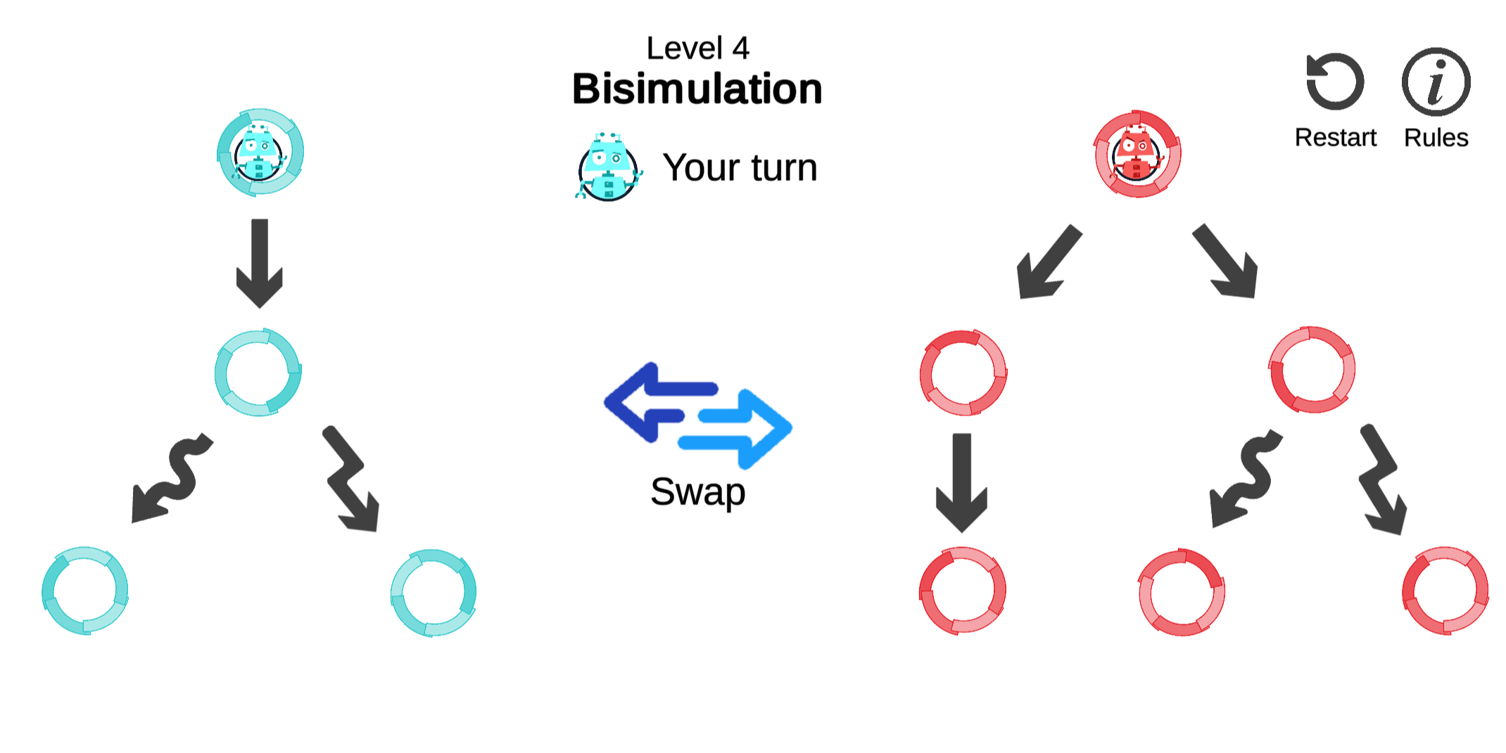
We now can add the bottom layer of Figure 2.1: That bisimilarity can be characterized through a game, where the defender wins if the game starts on a pair of bisimilar states. This approach has been popularized by Stirling (1996).

Definition 2.22 (Bisimulation Game) For a transition system $\mathcal{S}$, the bisimulation game ${\mathcal{G}}_\mathrm{B}^{\mathcal{S}}$ is played on attack positions $G^\mathrm{B}_{\mathrm{a}}≔ \mathcal{P}× \mathcal{P}$ and defense positions $G^\mathrm{B}_{\mathrm{d}}≔ \mathit{Act}× \mathcal{P}× \mathcal{P}$ with the following moves:⁴⁶

locale Equivalence_Games.bisim_game

• The attacker may swap sides $$[p, q] \quad \mathrel{\smash{›\!\!\frac{\;\enspace\;}{}\!\!›}}_\mathrm{B} \quad [q, p],$$
• or challenge simulation $$[p, q] \quad \mathrel{\smash{›\!\!\frac{\;\enspace\;}{}\!\!›}}_\mathrm{B} \quad (α, p', q) \quad \text{if} \quad p \xrightarrow{\smash{\raisebox{-2pt}{$\scriptstyle{α}$}}} p';$$
• and the defender answers simulation challenges $$(α, p', q) \quad \mathrel{\smash{›\!\!\frac{\;\enspace\;}{}\!\!›}}_\mathrm{B} \quad [p', q'] \quad \text{if} \quad q \xrightarrow{\smash{\raisebox{-2pt}{$\scriptstyle{α}$}}} q'.$$

A schematic depiction of the game rules can be seen in Figure 2.9. From dashed nodes, the game proceeds analogously to the initial attacker position.

Figure 2.9: Game scheme of the bisimulation game (Definition 2.22).

Example 2.15 Consider $\mathsf{p_{even}} \sim_\mathrm{B} \mathsf{p_{odd}}$ of Example 2.7. The bisimulation game on this system is given by Figure 2.10:

Figure 2.10: Bisimulation game under $\mathsf{p_{even}}, \mathsf{p_{odd}}$. Moves are annotated with the game rules from which they derive.

Clearly, there is no way for the attacker to get the defender stuck. Whatever strategy the attacker chooses, the game will go on forever, leading to a win for the defender. That it is always safe for the defender to answer with moves to $[\mathsf{p_{even}}, \mathsf{p_{odd}}]$ and $[\mathsf{p_{odd}}, \mathsf{p_{even}}]$ corresponds to $\mathcal{R} ≔ \{(\mathsf{p_{even}}, \mathsf{p_{odd}}), (\mathsf{p_{odd}}, \mathsf{p_{even}})\}$ being a bisimulation.

Example 2.16 Let us recall Example 2.6 of the “trolled philosophers,” where we determined $\mathsf{Q}$ and $\mathsf{T}$ to be non-bisimilar. The bisimulation game graph for the system is depicted in Figure 2.11.

The attacker can win by moving $[\mathsf{Q}, \mathsf{T}] \mathrel{\smash{›\!\!\frac{\;\enspace\;}{}\!\!›}}_\mathrm{B} [\mathsf{T}, \mathsf{Q}] \mathrel{\smash{›\!\!\frac{\;\enspace\;}{}\!\!›}}_\mathrm{B} (\tau, \mathsf{q_3}, \mathsf{Q}) \mathrel{\smash{›\!\!\frac{\;\enspace\;}{}\!\!›}}_\mathrm{B} [\mathsf{q_3}, \mathsf{q_{AB}}] \mathrel{\smash{›\!\!\frac{\;\enspace\;}{}\!\!›}}_\mathrm{B} [\mathsf{q_{AB}}, \mathsf{q_3}] \mathrel{\smash{›\!\!\frac{\;\enspace\;}{}\!\!›}}_\mathrm{B} (\mathsf{a}, \mathsf{q_1}, \mathsf{q_3}) \mathrel{\smash{{›/\!\!\!\!\frac{\;\enspace\;}{\;}\!\!›}}}_\mathrm{B}$. Along this sequence of positions, the defender never has a choice and is stuck in the end. The attacker exploits, that $\mathsf{T}$ can reach an early deadlock via $\mathsf{T} \xrightarrow{\smash{\raisebox{-2pt}{$\scriptstyle{\tau}$}}} \mathsf{q_{3}}$.

Figure 2.11: Bisimulation game on non-bisimilar states $\mathsf{Q}$ and $\mathsf{T}$ of Example 2.16. Moves are labeled by their justification. Defender-won positions are tinted blue.

Theorem 2.2 (Stirling’s Game Characterization) The defender wins the bisimulation game ${\mathcal{G}}_\mathrm{B}^{\mathcal{S}}$ starting at attacker position $[p, q]$ precisely if $p \sim_\mathrm{B} q$.⁴⁷

theorem Equivalence_Games.bisim_game.bisim_game_characterization

Proof. Sketch for both directions:

• If $\mathcal{R}$ is a symmetric simulation with $(p,q) ∈ \mathcal{R}$, then the following positional defender strategy is well-defined and winning from $[p, q]$:⁴⁸ $$s (α, p', q) ≔ [p', \operatorname{choose} q'\ldotp (p', q') ∈ \mathcal{R} \land q \xrightarrow{\smash{\raisebox{-2pt}{$\scriptstyle{α}$}}} q'].$$
• If there is a positional defender strategy $s$ winning from $[p, q]$, then the following relation $\mathcal{R_s}$ with $(p_0,q_0) ∈ \mathcal{R_s}$ is a symmetric simulation:⁴⁹ $$\mathcal{R_s} ≔ \{(p,q) \mid \text{there is a play $(p_0, q_0),\dots,(p,q)$ following strategy $s$}\}.$$

lemma Equivalence_Games.bisim_game.bisim_implies_defender_winning_strategy

lemma Equivalence_Games.bisim_game.defender_winning_strategy_implies_bisim

Remark 2.4. One of the big advantages of game characterizations is that they provide a way to discuss equivalence and inequivalence interactively among humans. There also are several computer game implementations of bisimulation games.

Figure 2.12: Screenshot of Peacock’s bisimulation computer game.

For instance, Peacock (2020) implements a game about simulation and bisimulation as well as several weaker notions. The human plays the attacker trying to point out the inequivalence of systems according to the rules of Definition 2.22. Figure 2.12 shows a screenshot of said game. It can be played on https://www.concurrency-theory.org/rvg-game/.

Example 2.17 If one plays the bisimulation game of Definition 2.22 without the swapping moves, it will characterize the simulation preorder.

Consider the family of processes $\mathsf{N}_n$ with $n \in \mathbb{N}$. Define $\mathsf{N}_0 := \mathbf{0}$ and $\mathsf{N}_{n + 1} := \mathsf{a}\ldotp\! \mathsf{N}_n$. Then, the simulation game played from $[\mathsf{N}_{n}, \mathsf{N}_{m}]$ is isomorphic to the $\leq$-game $\mathcal{G}_{\mathsf{leq}}$ from Example 2.13.

In this sense, comparisons of programs and of numbers are … comparable.

2.4.4 How Bisimulation Game and HML Are Connected

Let us pause to think how bisimulation game and Hennessy–Milner logic connect.

You might have wondered why we even need a dedicated bisimulation game. The Hennessy–Milner theorem implies that we could directly use the HML game of Definition 2.21 to decide bisimilarity:

Definition 2.23 (Naive Bisimulation Game) We extend the Definition 2.21 by the following prefix:

1. To challenge $[p,q]$, the attacker picks a formula $φ ∈ \mathsf{HML}$ (claiming that $φ$ distinguishes the states) and yields to the defender $(φ, p, q)$.
2. The defender decides where to start the HML game:
   1. Either at $(p, \neg φ)$ (claiming $φ$ to be non-distinguishing because it is untrue for $p$)
   2. or at $(q, φ)$ (claiming $φ$ to be non-distinguishing because it is true for $q$).
3. After that the turns proceed as prescribed by Definition 2.21.

This naive game, too, has the property that the defender wins from $[p,q]$ iff $p \sim_\mathrm{B} q$. The downside of the game is that the attacker has infinitely many options $φ ∈ \mathsf{HML}$ to pick from!

The proper bisimulation game of Definition 2.22, on the other hand, is finite for finite transition systems. Therefore, it induces decision procedures.

We will now argue that the bisimulation game actually is a variant of the naive game, where (1) the attacker names their formula gradually, and (2) the formulas stem from $\mathcal{O}^{}_{\mathrm{\lfloor B \rfloor}} \subseteq \mathsf{HML}$ of Definition 2.16. To this end, we will show that attacker’s winning strategies imply distinguishing formulas, and that a distinguishing formula from $\mathcal{O}^{}_{\mathrm{\lfloor B \rfloor}}$ certifies the existence of winning attacker strategies.

Example 2.18 Let us illustrate how to derive distinguishing formulas using the game of Example 2.16.

Recall that the attacker wins by moving $[\mathsf{Q}, \mathsf{T}] \mathrel{\smash{›\!\!\frac{\;\enspace\;}{}\!\!›}}_\mathrm{B} [\mathsf{T}, \mathsf{Q}] \mathrel{\smash{›\!\!\frac{\;\enspace\;}{}\!\!›}}_\mathrm{B} (\tau, \mathsf{q_3}, \mathsf{Q}) \mathrel{\smash{›\!\!\frac{\;\enspace\;}{}\!\!›}}_\mathrm{B} [\mathsf{q_3}, \mathsf{q_{AB}}] \mathrel{\smash{›\!\!\frac{\;\enspace\;}{}\!\!›}}_\mathrm{B} [\mathsf{q_{AB}}, \mathsf{q_3}] \mathrel{\smash{›\!\!\frac{\;\enspace\;}{}\!\!›}}_\mathrm{B} (\mathsf{a}, \mathsf{q_1}, \mathsf{q_3}) \mathrel{\smash{{›/\!\!\!\!\frac{\;\enspace\;}{\;}\!\!›}}}_\mathrm{B}$. In Figure 2.13, we label the game nodes with the (sub-)formulas this strategy corresponds to. Swap moves become negations, and simulation moves become observations with a conjunction of formulas for each defender option. This attacker strategy can thus be expressed by $\neg\langle \tau \rangle\textstyle\bigwedge \{\neg\langle \mathsf{a} \rangle\top\} \in \mathcal{O}^{}_{\mathrm{\lfloor B \rfloor}}$.

Figure 2.13: The bisimulation game of Example 2.18 with attacker formulas.

More generally, the following lemma explains the construction of distinguishing formulas from attacker strategies:

Lemma 2.9 Let $s$ be a positional winning strategy for the attacker on ${\mathcal{G}}_\mathrm{B}$ from $[p,q]$. Construct formulas recursively from game positions, ${φ}_{\mathcal{s}}(g)$, as follows: $$φ_{s}([p,q]) ≔ \begin{cases} \neg φ_{s}([q,p]) & \text{if } s([p,q]) = [q,p] \\ \langle \alpha \rangle \textstyle\bigwedge \{ φ_{s}([p',q']) \mid q \xrightarrow{\smash{\raisebox{-2pt}{$\scriptstyle{\alpha}$}}} q' \} & \text{if } s([p,q]) = (\alpha,p',q) \end{cases}$$ Then $φ_{s}([p,q])$ is well-defined and distinguishes $p$ from $q$. Also, $φ_{s}([p,q]) ∈ \mathcal{O}^{}_{\mathrm{\lfloor B \rfloor}}$.

Proof.

1. The given construction is well-defined as $s$ must induce a well-founded order on game positions in order for the attacker to win, and the recursive invocations remain in the attacker winning strategy.

2. The distinction can be derived by induction on the construction of $φ_{s}([p,q])$: Assume for $p',q'$ appearing in recursive invocations of the definition of $φ_{s}$ that $φ_{s}([p', q'])$ distinguishes them and that $φ_{s}([p', q']) ∈ \mathcal{O}^{}_{\mathrm{\lfloor B \rfloor}}$. We have to show that the constructions in $φ_{s}$ still fulfill this property:

   • As $φ_{s}([p',q'])$ distinguishes $p'$ from $q'$, its negation $\neg φ_{s}([p',q'])$ must distinguish $q'$ from $p'$ by the HML semantics. Moreover, the grammar of Definition 2.21 is closed under negation.
   • For $\langle \alpha \rangle \textstyle\bigwedge \{ φ_{s}([p',q']) \mid q \xrightarrow{\smash{\raisebox{-2pt}{$\scriptstyle{\alpha}$}}} q' \}$ to distinguish $p$ from $q$, there must be $p \xrightarrow{\smash{\raisebox{-2pt}{$\scriptstyle{\alpha}$}}} p^* \in \llbracket \textstyle\bigwedge \{ φ_{s}([p',q']) \mid q \xrightarrow{\smash{\raisebox{-2pt}{$\scriptstyle{\alpha}$}}} q' \} \rrbracket$, and for all $q^*$ with $q \xrightarrow{\smash{\raisebox{-2pt}{$\scriptstyle{\alpha}$}}} q^*$ it must be that $q^* \notin \llbracket \textstyle\bigwedge \{ φ_{s}([p',q']) \mid q \xrightarrow{\smash{\raisebox{-2pt}{$\scriptstyle{\alpha}$}}} q' \} \rrbracket$. We choose $p^* = p'$, because, as $s$ is an attacker winning strategy, $s([p, q]) = (\alpha, p', q)$ is a valid move with $p \xrightarrow{\smash{\raisebox{-2pt}{$\scriptstyle{\alpha}$}}} p'$. Also, all $q'$ the defender may select in answers remain in the winning domain of the attacker, and we may use the induction hypothesis that $q' \notin \llbracket φ_{s}([p',q']) \rrbracket$. Therefore, for each $q^*$ there is a false conjunct with $q' = q^*$ in $\textstyle\bigwedge \{ φ_{s}([p',q']) \mid q \xrightarrow{\smash{\raisebox{-2pt}{$\scriptstyle{\alpha}$}}} q' \}$ that proves $q* \notin \llbracket \textstyle\bigwedge \{ φ_{s}([p',q']) \mid q \xrightarrow{\smash{\raisebox{-2pt}{$\scriptstyle{\alpha}$}}} q' \} \rrbracket$.

Lemma 2.10 If $φ ∈ \mathcal{O}^{}_{\mathrm{\lfloor B \rfloor}}$ distinguishes $p$ from $q$, then the attacker wins from $[p,q]$.

Proof. By induction on the derivation of $φ ∈ \mathcal{O}^{}_{\mathrm{\lfloor B \rfloor}}$ according to the definition from Definition 2.16 with arbitrary $p$ and $q$.

• Case $φ = \langle α \rangle \textstyle\bigwedge_{i \in I} φ_i$. As $φ$ distinguishes $p$ from $q$, there must be a $p'$ such that $p \xrightarrow{\smash{\raisebox{-2pt}{$\scriptstyle{α}$}}} p'$ and that $\textstyle\bigwedge_{i \in I} φ_i$ distinguishes $p'$ from every $q' \in \operatorname{Der}(q, α)$. That is, for each $q' \in \operatorname{Der}(q, α)$, at least one $φ_i \in \mathcal{O}^{}_{\mathrm{\lfloor B \rfloor}}$ must be false. By induction hypothesis, the attacker thus wins each $[p',q']$. As these attacker positions encompass all successors of $(α, p', q)$, the attacker also wins this defender position and can win from $[p,q]$ by moving there with a simulation challenge.
• Case $φ = \neg φ'$. As $φ$ distinguishes $p$ from $q$, $φ'$ distinguishes $q$ from $p$. By induction hypothesis, the attacker wins $[q, p]$. So they can also win $[p, q]$ by performing a swap.

Lemma 2.9 and Lemma 2.10, together with the fact that $\mathcal{O}^{}_{\mathrm{\lfloor B \rfloor}}$ and $\mathsf{HML}$ are equally distinctive (Lemma 2.7), yield:

Theorem 2.3 The attacker wins ${\mathcal{G}}_\mathrm{B}$ from $[p,q]$ precisely if there is $φ ∈ \mathsf{HML}$ distinguishing $p$ from $q$.

Of course, we already knew this! Theorem 2.3 is just another way of gluing together the Hennessy–Milner theorem on bisimulation (Theorem 2.1) and Stirling’s bisimulation game characterization (Theorem 2.2), modulo the determinacy of games. We thus have added the last arrow on the right side of Figure 2.1.

2.4.5 Deciding Reachability Games

All we need to turn a game characterization into a decision procedure, is a way to decide which player wins a position. Algorithm 2.1 describes how to compute who wins a finite reachability game for each position in time linear to the size of the game graph $\left|\mathrel{\smash{›\!\!\frac{\;\enspace\;}{}\!\!›}}\right|$.

$$\begin{array}{lr} \operatorname{\mathbf{def}}\; \mathtt{compute\_winning\_region}(\mathcal{G}=(G,G_{\mathrm{d}},\mathrel{\smash{›\!\!\frac{\;\enspace\;}{}\!\!›}})) \colon & \\ \quad \mathtt{defender\_options} := [g \mapsto n \mid g \in G \land n = \left|\{g' \mid g \mathrel{\smash{›\!\!\frac{\;\enspace\;}{}\!\!›}}g'\}\right|] & \\ \quad \mathtt{attacker\_win} := \varnothing & \\ \quad \mathtt{todo} := \{g\in G_{\mathrm{d}}\mid \mathtt{defender\_options}[g]=0\} & \\ \quad \operatorname{\mathbf{while}}\; \mathtt{todo} \neq \varnothing \colon & \\ \quad \quad \mathtt{g} := \operatorname{\mathbf{some}}\; \mathtt{todo} & \\ \quad \quad \mathtt{todo} := \mathtt{todo} \mathbin{\backslash}\{\mathtt{g}\} & \\ \quad \quad \operatorname{\mathbf{if}}\; \mathtt{g} \notin \mathtt{attacker\_win} \colon & \\ \quad \quad \quad \mathtt{attacker\_win} := \mathtt{attacker\_win} \cup \{\mathtt{g}\} & \\ \quad \quad \quad \operatorname{\mathbf{for}}\; \mathtt{g_{p}} \in (\cdot \mathrel{\smash{›\!\!\frac{\;\enspace\;}{}\!\!›}}\mathtt{g}) \colon & \\ \quad \quad \quad \quad \mathtt{defender\_options}[\mathtt{g_{p}}]:=\mathtt{defender\_options}[\mathtt{g_{p}}]-1 & \\ \quad \quad \quad \quad \operatorname{\mathbf{if}}\; \mathtt{g_{p}} \in G_{\mathrm{a}}\lor \mathtt{defender\_options}[\mathtt{g_{p}}]=0 \colon & \\ \quad \quad \quad \quad \quad \mathtt{todo} := \mathtt{todo} \cup \{\mathtt{g_{p}}\} & \\ \quad \mathsf{Win}_\mathrm{a}:= \mathtt{attacker\_win} & \\ \quad \operatorname{\mathbf{return}}\; \mathsf{Win}_\mathrm{a}& \\ \end{array}$$

Algorithm 2.1: Algorithm for deciding the attacker winning region $\mathsf{Win}_\mathrm{a}$ of a reachability game $\mathcal{G}$ in linear time of $\left|\mathrel{\smash{›\!\!\frac{\;\enspace\;}{}\!\!›}}\right|$ and linear space of $\left|G\right|$.

Intuitively, $\mathtt{compute\_winning\_region}$ first assumes that the defender were to win everywhere and that each outgoing move of every position might be a winning option for the defender. Over time, every position that is determined to be lost by the defender is added to a $\mathtt{todo}$ list.⁵⁰

⁵⁰  Variants of this algorithm and explanation have also been used in Bisping (2018) and Bisping et al. (2022).

At first, the defender loses immediately exactly at the defender’s dead-ends. Each defender-lost position is added to the $\mathtt{attacker\_win}$ set. To trigger the recursion, each predecessor is noted as defender-lost, if it is controlled by the attacker, or the amount of outgoing defender options is decremented if the predecessor is defender-controlled. If the count of a predecessor position hits 0, the defender also loses from there.

Once we run out of $\mathtt{todo}$ positions, we know that the attacker has winning strategies exactly for each position we have visited.

The following Table 2.1 lists how Algorithm 2.1 computes the winning region $\mathsf{Win}_\mathrm{a}= \{[\mathsf{2a}], (\mathsf{3})\}$ of the game of Definition 2.16.

Table 2.1: Solving the game of Definition 2.16

$\mathtt{g}$	$\mathtt{defender\_options}$	$\mathtt{todo}$
-	$(\mathsf{1}) \mapsto 2$, $(\mathsf{3}) \mapsto 0$	$(\mathsf{3})$
$(\mathsf{3})$	$(\mathsf{1}) \mapsto 2$, $(\mathsf{3}) \mapsto 0$	$[\mathsf{2a}]$
$[\mathsf{2a}]$	$(\mathsf{1}) \mapsto 1$, $(\mathsf{3}) \mapsto 0$	$\varnothing$

The inner loop of Algorithm 2.1 clearly can run at most $\left|\mathrel{\smash{›\!\!\frac{\;\enspace\;}{}\!\!›}}\right|$-many times. Using sufficiently clever data structures, the algorithm thus shows:

Proposition 2.9 Given a finite reachability game $\mathcal{G}=(G,G_{\mathrm{d}},\mathrel{\smash{›\!\!\frac{\;\enspace\;}{}\!\!›}})$, the attacker’s winning region $\mathsf{Win}_\mathrm{a}$ (and $\mathsf{Win}_\mathrm{d}$ as well) can be computed in $\mathit{O}(\left|\mathrel{\smash{›\!\!\frac{\;\enspace\;}{}\!\!›}}\right|)$ time and $\mathit{O}(\left|G\right|)$ space.

2.5 Discussion

This chapter has taken a tour of characterizations for standard notions of behavioral preorder and equivalence on transition systems such as trace equivalence and bisimilarity.

In particular, in constructing the relationships of Figure 2.1 for bisimilarity, we have collected the theoretical ingredients for a certifying algorithm to check bisimilarity of states.

Figure 2.14: Checking bisimilarity and providing certificates.

Figure 2.14 describes how to not only answer the question whether two states $p$ and $q$ are bisimilar, but how to also either provide a bisimulation relation or a distinguishing formula for the two as certificates for the answer. (The arrows stand for computations, the boxes for data.)

In this view, the game of possible distinctions and their preventability between attacker and defender serves as the “ground truth” about the bisimilarity of two states. Bisimulation relations and modal formulas only appear as witnesses of defender and attacker strategies, mediating between game and transition system. The Hennessy–Milner theorem emerges on this level as a shadow of the determinacy of the bisimulation game (Idea 2.1). This whole framework draws heavily from Stirling (1996).

We have disregarded the topic of axiomatic characterizations for behavioral equivalences. In these, sets of equations on process algebra terms (such as $\textsf{CCS}$) define behavioral congruences. Thus, they tend to be coupled to specific process languages and lack the genericity we pursue in starting out from transition systems.

We have observed that behavioral equivalences can be arranged in hierarchies and that these hierarchies could be handled nicely using modal characterizations to rank distinguishing powers (Subsection 2.3.3). We have also seen how to link game rules to productions in a language of potentially distinguishing formulas (Subsection 2.4.4). This departs from common textbook presentations that motivate the bisimulation game through the relational (coinductive) characterization (e.g. Sangiorgi, 2012). In later chapters, we will rather derive equivalence games from grammars of modal formulas (Idea 2.2), to generalize the framework of Figure 2.14 for whole spectra of equivalences.

But first, we have to make formal what we mean by equivalence spectra.

Bisping, B. (2018). Computing coupled similarity [Master’s thesis, Technische Universität Berlin]. https://coupledsim.bbisping.de/bisping_computingCoupledSimilarity_thesis.pdf

Bisping, B., Jansen, D. N., & Nestmann, U. (2022). Deciding All Behavioral Equivalences at Once: A Game for Linear-Time–Branching-Time Spectroscopy. Logical Methods in Computer Science, 18(3). https://doi.org/10.46298/lmcs-18(3:19)2022

Gale, D., & Stewart, F. M. (1953). Infinite games with perfect information. In H. W. Kuhn & A. W. Tucker (Eds.), Contributions to the theory of games, volume II (pp. 245–266). Princeton University Press. https://doi.org/10.1515/9781400881970-014

Gazda, M., Fokkink, W., & Massaro, V. (2020). Congruence from the operator’s point of view: Syntactic requirements on modal characterizations. Acta Informatica, 57(3–5), 329–351. https://doi.org/10.1007/s00236-019-00355-5

Hennessy, M., & Milner, R. (1980). On observing nondeterminism and concurrency. In J. W. de Bakker & J. van Leeuwen (Eds.), Automata, languages and programming (Vol. 85, pp. 299–309). Springer. https://doi.org/10.1007/3-540-10003-2_79

Milner, R. (1980). A calculus of communicating systems (Vol. 92). Springer. https://doi.org/10.1007/3-540-10235-3

Peacock, D. A. (2020). Process equivalences as a video game [Bachelor's Thesis, Technische Universität Berlin]. https://drive.google.com/drive/folders/19YuOCXI_7CEB4p9fgr6kDKCTbFwx2VU9

Sangiorgi, D. (2012). Introduction to bisimulation and coinduction. Cambridge University Press. https://doi.org/10.1017/CBO9780511777110

Stirling, C. (1996). Modal and temporal logics for processes. In F. Moller & G. Birtwistle (Eds.), Logics for concurrency: Structure versus automata (Vol. 1043, pp. 149–237). Springer. https://doi.org/10.1007/3-540-60915-6_5

Wortmann, J. K., Olesen, S. R., & Enevoldsen, S. (2015). CAAL 2.0 – recursive HML, distinguishing formulae, equivalence collapses and parallel fixed-point computations (Vol. DES103F15). Aalborg University. https://caal.cs.aau.dk/docs/CAAL2_RDEP.pdf

Zielonka, W. (1998). Infinite games on finitely coloured graphs with applications to automata on infinite trees. Theoretical Computer Science, 200(1), 135–183. https://doi.org/https://doi.org/10.1016/S0304-3975(98)00009-7